24 A polyphase circuit

mayeb a new title: superposition and polyphase

combining two topics

Abstract

A circuit to illustrate superposition and polyphase circuit analysis.

24.1 Introduction

what is superposition what is a polyphase circuit.

as discussed below too large for useful symbolic analysis.

What is a phasor?

Phasor

In physics and engineering, a phasor (a portmanteau of phase vector[1][2]) is a complex number representing a sinusoidal function whose amplitude (A), and initial phase (θ) are time-invariant and whose angular frequency (ω) is fixed. It is related to a more general concept called analytic representation,[3] which decomposes a sinusoid into the product of a complex constant and a factor depending on time and frequency. The complex constant, which depends on amplitude and phase, is known as a phasor, or complex amplitude,[4][5] and (in older texts) sinor[6] or even complexor.[6

A common application is in the steady-state analysis of an electrical network powered by time varying current where all signals are assumed to be sinusoidal with a common frequency. Phasor representation allows the analyst to represent the amplitude and phase of the signal using a single complex number. The only difference in their analytic representations is the complex amplitude (phasor). A linear combination of such functions can be represented as a linear combination of phasors (known as phasor arithmetic or phasor algebra[7]: 53 ) and the time/frequency dependent factor that they all have in common.

Charles Proteus Steinmetz

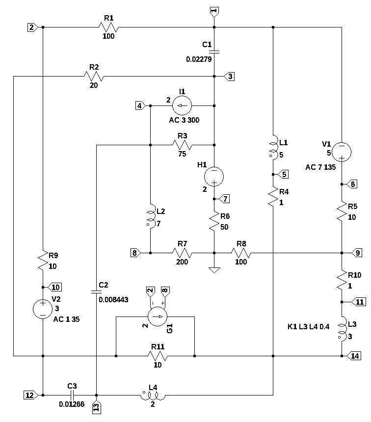
24.2 Circuit description

The most commen every day poly phase circuits are three phase power circuits for the electric utility. In this example there thre three phases and three frequencies. To illustrate supper posistion .

a collection of AC and DC sources
coupled inductors
dependent sources
RLC
non planer

too large to do by hand, can’t simplify, not planar, so loop analysis is difficult. But also too large for symbolic solution.

source	DC	Magnitude @ angle	frequency, Hz
V1	5	7 @ 135	3
V2	1	1 @ 35	5
I1	2	3 @ 300	7

source	DC	AC, mag @ phase	omega
V1	5	7 @ 135	\(2 \pi 3\)
V2	1	1 @ 35	\(2 \pi 5\)
I1	2	3 @ 300	\(2 \pi 7\)

Independent sources get set to zero one at a time for each frequency.

V is zero because is an AC short and I is zero because no current flows and is open.

Superposition theorem

What is the Superposition Theorem?

The strategy used in the superposition theorem is to eliminate all but one source of power within a network at a time. Then, we use series and parallel circuit analysis techniques to determine voltage drops and currents within the modified network for each power source separately.

This process is then repeated sequentially by individually evaluating the circuit for every voltage and current source in the system. After each individual analysis has been completed, the voltage and current values are all “superimposed” on top of each other (added algebraically) to find the actual voltage drops and currents with all sources active.

What does it mean to turn off a current source? It means we set ‍

. That’s the same as replacing the current source with an open circuit.

What does it mean to turn off a voltage source? It means we set ‍

. This is the same thing as replacing the voltage source or battery by a short circuit.

The theorem does not apply to non-linear circuits. The requisite of linearity indicates that the superposition theorem is only applicable to determine voltage and current but not power. Power dissipation is a nonlinear function that does not algebraically add to an accurate total when only one source is considered at a time.

Superposition works for voltage and current but not power. In other words, the sum of the powers of each source with the other sources turned off is not the real consumed power. To calculate power we first use superposition to find both current and voltage of each linear element and then calculate the sum of the multiplied voltages and currents.

24.3 Circuit description

V1 6 1 5 AC 7 90
V2 10 12 1 AC 1 35
I3 3 4 2 AC 3 210
L3 11 14 3 Rser=0
L1 1 5 5 Rser=0
L4 14 13 2 Rser=0
L2 4 8 7 Rser=0
H1 7 3 V2 2
G1 12 14 8 2 2
C1 3 1 0.02279
C2 4 13 0.008443
C3 13 12 0.01266
R9 2 10 10
R6 7 0 50
R4 5 14 1
R1 1 2 100
R3 3 4 75
R7 0 8 200
R11 14 12 10
R5 6 9 10
R10 9 11 1
R8 9 0 100
R2 3 12 20
K1 L3 L4 0.4

import os
from sympy import *
import numpy as np
from tabulate import tabulate
from scipy import signal
import matplotlib.pyplot as plt
import pandas as pd
import SymMNA
init_printing()

In electrical engineering, a time invarient sinusudial signal can be represented either by polar or rectangular notation. The function polar converts the polar representation, also called a phasor to rectangular notation.

def polar(mag, ang, units='deg'):
    ''' polar to rectangular conversion
        mag: float
            magnitude of the time invarient sinusudial signal
        ang: float
            the angle of the time invarient sinusudial signal
        units: string
            if units is set to deg, and is in degrees not radians
    '''
    if units == 'deg':
        ang = ang * np.pi / 180
    return mag * np.exp(1j * ang)

24.4 Symbolic MNA code

24.5 Load the net list

independent sources have their values set to the DC value.

example_net_list = '''
V1 6 1 5 
V2 10 12 1 
I3 3 4 2 
L3 11 14 3 
L1 1 5 5 
L4 14 13 2 
L2 4 8 7 
H1 7 3 V2 2
G1 12 14 8 2 2
C1 3 1 0.02279
C2 4 13 0.008443
C3 13 12 0.01266
R9 2 10 10
R6 7 0 50
R4 5 14 1
R1 1 2 100
R3 3 4 75
R7 0 8 200
R11 14 12 10
R5 6 9 10
R10 9 11 1
R8 9 0 100
R2 3 12 20
K1 L3 L4 0.4
'''

report, df, df2, A, X, Z = SymMNA.smna(example_net_list)

print(report)

Net list report
number of lines in netlist: 24
number of branches: 23
number of nodes: 14
number of unknown currents: 7
number of RLC (passive components): 18
number of inductors: 4
number of independent voltage sources: 2
number of independent current sources: 1
number of op amps: 0
number of E - VCVS: 0
number of G - VCCS: 1
number of F - CCCS: 0
number of H - CCVS: 1
number of K - Coupled inductors: 1

# Put matricies into SymPy 
X = Matrix(X)
Z = Matrix(Z)

equ = Eq(A*X,Z)

equ

\(\displaystyle \left[\begin{matrix}- C_{1} s v_{3} + I_{L1} - I_{V1} + v_{1} \left(C_{1} s + \frac{1}{R_{1}}\right) - \frac{v_{2}}{R_{1}}\\v_{2} \cdot \left(\frac{1}{R_{9}} + \frac{1}{R_{1}}\right) - \frac{v_{10}}{R_{9}} - \frac{v_{1}}{R_{1}}\\- C_{1} s v_{1} - I_{H1} + v_{3} \left(C_{1} s + \frac{1}{R_{3}} + \frac{1}{R_{2}}\right) - \frac{v_{4}}{R_{3}} - \frac{v_{12}}{R_{2}}\\- C_{2} s v_{13} + I_{L2} + v_{4} \left(C_{2} s + \frac{1}{R_{3}}\right) - \frac{v_{3}}{R_{3}}\\- I_{L1} - \frac{v_{14}}{R_{4}} + \frac{v_{5}}{R_{4}}\\I_{V1} + \frac{v_{6}}{R_{5}} - \frac{v_{9}}{R_{5}}\\I_{H1} + \frac{v_{7}}{R_{6}}\\- I_{L2} + \frac{v_{8}}{R_{7}}\\v_{9} \cdot \left(\frac{1}{R_{8}} + \frac{1}{R_{5}} + \frac{1}{R_{10}}\right) - \frac{v_{6}}{R_{5}} - \frac{v_{11}}{R_{10}}\\I_{V2} + \frac{v_{10}}{R_{9}} - \frac{v_{2}}{R_{9}}\\I_{L3} + \frac{v_{11}}{R_{10}} - \frac{v_{9}}{R_{10}}\\- C_{3} s v_{13} - I_{V2} - g_{1} v_{2} + g_{1} v_{8} + v_{12} \left(C_{3} s + \frac{1}{R_{2}} + \frac{1}{R_{11}}\right) - \frac{v_{3}}{R_{2}} - \frac{v_{14}}{R_{11}}\\- C_{2} s v_{4} - C_{3} s v_{12} - I_{L4} + v_{13} \left(C_{2} s + C_{3} s\right)\\- I_{L3} + I_{L4} + g_{1} v_{2} - g_{1} v_{8} + v_{14} \cdot \left(\frac{1}{R_{4}} + \frac{1}{R_{11}}\right) - \frac{v_{5}}{R_{4}} - \frac{v_{12}}{R_{11}}\\- v_{1} + v_{6}\\v_{10} - v_{12}\\- I_{L3} L_{3} s - I_{L4} M_{1} s + v_{11} - v_{14}\\- I_{L1} L_{1} s + v_{1} - v_{5}\\- I_{L3} M_{1} s - I_{L4} L_{4} s - v_{13} + v_{14}\\- I_{L2} L_{2} s + v_{4} - v_{8}\\- I_{V2} h_{1} - v_{3} + v_{7}\end{matrix}\right] = \left[\begin{matrix}0\\0\\- I_{3}\\I_{3}\\0\\0\\0\\0\\0\\0\\0\\0\\0\\0\\V_{1}\\V_{2}\\0\\0\\0\\0\\0\end{matrix}\right]\)

# turn the free symbols into SymPy variables
var(str(equ.free_symbols).replace('{','').replace('}',''))

\(\displaystyle \left( I_{H1}, \ L_{1}, \ v_{9}, \ I_{L1}, \ R_{1}, \ v_{13}, \ s, \ v_{4}, \ v_{5}, \ v_{10}, \ R_{9}, \ h_{1}, \ C_{2}, \ V_{2}, \ R_{4}, \ v_{11}, \ C_{1}, \ V_{1}, \ I_{V2}, \ I_{L3}, \ C_{3}, \ R_{5}, \ R_{11}, \ v_{2}, \ v_{7}, \ R_{3}, \ I_{L2}, \ v_{14}, \ R_{2}, \ v_{12}, \ R_{7}, \ L_{4}, \ R_{8}, \ v_{1}, \ L_{2}, \ g_{1}, \ v_{3}, \ R_{10}, \ v_{8}, \ I_{L4}, \ L_{3}, \ v_{6}, \ I_{3}, \ M_{1}, \ I_{V1}, \ R_{6}\right)\)

24.6 Symbolic solution

symbolic_solution = solve(equ,X)

24.7 Built a dictionary of element values

element_value_keys = []
element_value_values = []

for i in range(len(df)):
    if df.iloc[i]['element'][0] == 'F' or df.iloc[i]['element'][0] == 'E' or df.iloc[i]['element'][0] == 'G' or df.iloc[i]['element'][0] == 'H':
        element_value_keys.append(var(df.iloc[i]['element'].lower()))
        element_value_values.append(df.iloc[i]['value'])
        #print('{:s}:{:f},'.format(df.iloc[i]['element'].lower(),df.iloc[i]['value']))
    else:
        element_value_keys.append(var(df.iloc[i]['element']))
        element_value_values.append(df.iloc[i]['value'])
        #print('{:s}:{:.4e},'.format(df.iloc[i]['element'],df.iloc[i]['value']))

element_values = dict(zip(element_value_keys, element_value_values))

# calculate the coupling constant from the mutual inductance
element_values[M1] = element_values[K1]*np.sqrt(element_values[L3] *element_values[L4])
print('mutual inductance, M1 = {:.9f}'.format(element_values[M1]))

mutual inductance, M1 = 0.979795897

element_values

\(\displaystyle \left\{ C_{1} : 0.02279, \ C_{2} : 0.008443, \ C_{3} : 0.01266, \ I_{3} : 2.0, \ K_{1} : 0.4, \ L_{1} : 5.0, \ L_{2} : 7.0, \ L_{3} : 3.0, \ L_{4} : 2.0, \ M_{1} : 0.979795897113271, \ R_{1} : 100.0, \ R_{10} : 1.0, \ R_{11} : 10.0, \ R_{2} : 20.0, \ R_{3} : 75.0, \ R_{4} : 1.0, \ R_{5} : 10.0, \ R_{6} : 50.0, \ R_{7} : 200.0, \ R_{8} : 100.0, \ R_{9} : 10.0, \ V_{1} : 5.0, \ V_{2} : 1.0, \ g_{1} : 2.0, \ h_{1} : 2.0\right\}\)

element_values[I3]

\(\displaystyle 2.0\)

24.8 Operating point

equ_values = equ.subs(element_values)
equ_values

\(\displaystyle \left[\begin{matrix}I_{L1} - I_{V1} - 0.02279 s v_{3} + v_{1} \cdot \left(0.02279 s + 0.01\right) - 0.01 v_{2}\\- 0.01 v_{1} - 0.1 v_{10} + 0.11 v_{2}\\- I_{H1} - 0.02279 s v_{1} - 0.05 v_{12} + v_{3} \cdot \left(0.02279 s + 0.0633333333333333\right) - 0.0133333333333333 v_{4}\\I_{L2} - 0.008443 s v_{13} - 0.0133333333333333 v_{3} + v_{4} \cdot \left(0.008443 s + 0.0133333333333333\right)\\- I_{L1} - 1.0 v_{14} + 1.0 v_{5}\\I_{V1} + 0.1 v_{6} - 0.1 v_{9}\\I_{H1} + 0.02 v_{7}\\- I_{L2} + 0.005 v_{8}\\- 1.0 v_{11} - 0.1 v_{6} + 1.11 v_{9}\\I_{V2} + 0.1 v_{10} - 0.1 v_{2}\\I_{L3} + 1.0 v_{11} - 1.0 v_{9}\\- I_{V2} - 0.01266 s v_{13} + v_{12} \cdot \left(0.01266 s + 0.15\right) - 0.1 v_{14} - 2.0 v_{2} - 0.05 v_{3} + 2.0 v_{8}\\- I_{L4} - 0.01266 s v_{12} + 0.021103 s v_{13} - 0.008443 s v_{4}\\- I_{L3} + I_{L4} - 0.1 v_{12} + 1.1 v_{14} + 2.0 v_{2} - 1.0 v_{5} - 2.0 v_{8}\\- v_{1} + v_{6}\\v_{10} - v_{12}\\- 3.0 I_{L3} s - 0.979795897113271 I_{L4} s + v_{11} - v_{14}\\- 5.0 I_{L1} s + v_{1} - v_{5}\\- 0.979795897113271 I_{L3} s - 2.0 I_{L4} s - v_{13} + v_{14}\\- 7.0 I_{L2} s + v_{4} - v_{8}\\- 2.0 I_{V2} - v_{3} + v_{7}\end{matrix}\right] = \left[\begin{matrix}0\\0\\-2.0\\2.0\\0\\0\\0\\0\\0\\0\\0\\0\\0\\0\\5.0\\1.0\\0\\0\\0\\0\\0\end{matrix}\right]\)

equ_values_dc = equ_values.subs({s:0})
equ_values_dc  # display the equations

\(\displaystyle \left[\begin{matrix}I_{L1} - I_{V1} + 0.01 v_{1} - 0.01 v_{2}\\- 0.01 v_{1} - 0.1 v_{10} + 0.11 v_{2}\\- I_{H1} - 0.05 v_{12} + 0.0633333333333333 v_{3} - 0.0133333333333333 v_{4}\\I_{L2} - 0.0133333333333333 v_{3} + 0.0133333333333333 v_{4}\\- I_{L1} - 1.0 v_{14} + 1.0 v_{5}\\I_{V1} + 0.1 v_{6} - 0.1 v_{9}\\I_{H1} + 0.02 v_{7}\\- I_{L2} + 0.005 v_{8}\\- 1.0 v_{11} - 0.1 v_{6} + 1.11 v_{9}\\I_{V2} + 0.1 v_{10} - 0.1 v_{2}\\I_{L3} + 1.0 v_{11} - 1.0 v_{9}\\- I_{V2} + 0.15 v_{12} - 0.1 v_{14} - 2.0 v_{2} - 0.05 v_{3} + 2.0 v_{8}\\- I_{L4}\\- I_{L3} + I_{L4} - 0.1 v_{12} + 1.1 v_{14} + 2.0 v_{2} - 1.0 v_{5} - 2.0 v_{8}\\- v_{1} + v_{6}\\v_{10} - v_{12}\\v_{11} - v_{14}\\v_{1} - v_{5}\\- v_{13} + v_{14}\\v_{4} - v_{8}\\- 2.0 I_{V2} - v_{3} + v_{7}\end{matrix}\right] = \left[\begin{matrix}0\\0\\-2.0\\2.0\\0\\0\\0\\0\\0\\0\\0\\0\\0\\0\\5.0\\1.0\\0\\0\\0\\0\\0\end{matrix}\right]\)

U_dc = solve(equ_values_dc,X)
U_dc

\(\displaystyle \left\{ I_{H1} : -11.5738896073146, \ I_{L1} : 20.3047789474962, \ I_{L2} : 2.80469316139686, \ I_{L3} : 15.3718733304192, \ I_{L4} : 0.0, \ I_{V1} : -0.993290561707708, \ I_{V2} : -21.2980695092039, \ v_{1} : -1432.92537125407, \ v_{10} : 909.862274758366, \ v_{11} : -1453.23015020156, \ v_{12} : 908.862274758366, \ v_{13} : -1453.23015020156, \ v_{14} : -1453.23015020156, \ v_{2} : 696.881579666327, \ v_{3} : 621.290619384137, \ v_{4} : 560.938632279372, \ v_{5} : -1432.92537125407, \ v_{6} : -1427.92537125407, \ v_{7} : 578.694480365729, \ v_{8} : 560.938632279372, \ v_{9} : -1437.85827687114\right\}\)

table_header = ['unknown', 'mag','phase, deg']
table_row = []

for name, value in U_dc.items():
    table_row.append([str(name),float(abs(value)),float(arg(value)*180/np.pi)])

print(tabulate(table_row, headers=table_header,colalign = ('left','decimal','decimal'),tablefmt="simple",floatfmt=('5s','.6f','.6f')))

unknown            mag    phase, deg
---------  -----------  ------------
v1         1432.925371    180.000000
v2          696.881580      0.000000
v3          621.290619      0.000000
v4          560.938632      0.000000
v5         1432.925371    180.000000
v6         1427.925371    180.000000
v7          578.694480      0.000000
v8          560.938632      0.000000
v9         1437.858277    180.000000
v10         909.862275      0.000000
v11        1453.230150    180.000000
v12         908.862275      0.000000
v13        1453.230150    180.000000
v14        1453.230150    180.000000
I_V1          0.993291    180.000000
I_V2         21.298070    180.000000
I_L3         15.371873      0.000000
I_L1         20.304779      0.000000
I_L4          0.000000    nan
I_L2          2.804693      0.000000
I_H1         11.573890    180.000000

LTSpice results:

--- Operating Point ---
V(6):    -1427.93    voltage
V(1):    -1432.93    voltage
V(10):   909.862     voltage
V(12):   908.862     voltage
V(3):    621.291     voltage
V(4):    560.939     voltage
V(11):   -1453.23    voltage
V(14):   -1453.23    voltage
V(5):    -1432.93    voltage
V(13):   -1453.23    voltage
V(8):    560.939     voltage
V(7):    578.694     voltage
V(2):    696.882     voltage
V(9):    -1437.86    voltage
I(C1):   4.68156e-11     device_current
I(C2):   1.70056e-11     device_current
I(C3):   -2.99041e-11    device_current
I(H1):   -11.5739    device_current
I(L3):   15.3719     device_current
I(L1):   20.3048     device_current
I(L4):   -4.69091e-11    device_current
I(L2):   2.80469     device_current
I(I3):   2   device_current
I(R9):   -21.2981    device_current
I(R6):   11.5739     device_current
I(R4):   20.3048     device_current
I(R1):   -21.2981    device_current
I(R3):   0.804693    device_current
I(R7):   -2.80469    device_current
I(R11):  -236.209    device_current
I(R5):   0.993291    device_current
I(R10):  15.3719     device_current
I(R8):   -14.3786    device_current
I(R2):   -14.3786    device_current
I(G1):   -271.886    device_current
I(V1):   -0.993291   device_current
I(V2):   -21.2981    device_current

24.9 Independednt sources with the same frequency

ev_w = element_values.copy() # ev for element values

ev_w[I3] = polar(3, 300, units='deg')
ev_w[V2] = polar(1, 35, units='deg')
ev_w[V1] = polar(7, 135, units='deg')

ev_w

{V1: (-4.949747468305832+4.949747468305833j),
 V2: (0.8191520442889918+0.573576436351046j),
 I3: (1.5000000000000004-2.598076211353316j),
 L3: 3.0,
 L1: 5.0,
 L4: 2.0,
 L2: 7.0,
 h1: 2.0,
 g1: 2.0,
 C1: 0.02279,
 C2: 0.008443,
 C3: 0.01266,
 R9: 10.0,
 R6: 50.0,
 R4: 1.0,
 R1: 100.0,
 R3: 75.0,
 R7: 200.0,
 R11: 10.0,
 R5: 10.0,
 R10: 1.0,
 R8: 100.0,
 R2: 20.0,
 K1: 0.4,
 M1: 0.9797958971132712}

equ_ev_w = equ.subs(ev_w)

equ_ev_w = equ_ev_w.subs({s:2*np.pi*3j})

equ_ev_w

\(\displaystyle \left[\begin{matrix}I_{L1} - I_{V1} + v_{1} \cdot \left(0.01 + 0.429581379451868 i\right) - 0.01 v_{2} - 0.429581379451868 i v_{3}\\- 0.01 v_{1} - 0.1 v_{10} + 0.11 v_{2}\\- I_{H1} - 0.429581379451868 i v_{1} - 0.05 v_{12} + v_{3} \cdot \left(0.0633333333333333 + 0.429581379451868 i\right) - 0.0133333333333333 v_{4}\\I_{L2} - 0.159146800645552 i v_{13} - 0.0133333333333333 v_{3} + v_{4} \cdot \left(0.0133333333333333 + 0.159146800645552 i\right)\\- I_{L1} - 1.0 v_{14} + 1.0 v_{5}\\I_{V1} + 0.1 v_{6} - 0.1 v_{9}\\I_{H1} + 0.02 v_{7}\\- I_{L2} + 0.005 v_{8}\\- 1.0 v_{11} - 0.1 v_{6} + 1.11 v_{9}\\I_{V2} + 0.1 v_{10} - 0.1 v_{2}\\I_{L3} + 1.0 v_{11} - 1.0 v_{9}\\- I_{V2} + v_{12} \cdot \left(0.15 + 0.238635377966681 i\right) - 0.238635377966681 i v_{13} - 0.1 v_{14} - 2.0 v_{2} - 0.05 v_{3} + 2.0 v_{8}\\- I_{L4} - 0.238635377966681 i v_{12} + 0.397782178612232 i v_{13} - 0.159146800645552 i v_{4}\\- I_{L3} + I_{L4} - 0.1 v_{12} + 1.1 v_{14} + 2.0 v_{2} - 1.0 v_{5} - 2.0 v_{8}\\- v_{1} + v_{6}\\v_{10} - v_{12}\\- 56.5486677646163 i I_{L3} - 18.4687175543308 i I_{L4} + v_{11} - v_{14}\\- 94.2477796076938 i I_{L1} + v_{1} - v_{5}\\- 18.4687175543308 i I_{L3} - 37.6991118430775 i I_{L4} - v_{13} + v_{14}\\- 131.946891450771 i I_{L2} + v_{4} - v_{8}\\- 2.0 I_{V2} - v_{3} + v_{7}\end{matrix}\right] = \left[\begin{matrix}0\\0\\-1.5 + 2.59807621135332 i\\1.5 - 2.59807621135332 i\\0\\0\\0\\0\\0\\0\\0\\0\\0\\0\\-4.94974746830583 + 4.94974746830583 i\\0.819152044288992 + 0.573576436351046 i\\0\\0\\0\\0\\0\end{matrix}\right]\)

U_w = solve(equ_ev_w,X)
U_w

\(\displaystyle \left\{ I_{H1} : -0.153544437655104 - 0.0892500106463104 i, \ I_{L1} : 3.54302617527629 + 2.81001510230497 i, \ I_{L2} : 0.945703908332592 + 0.362574674184583 i, \ I_{L3} : 10.4231744502691 + 8.54663272904898 i, \ I_{L4} : -18.259482746311 - 6.1397795231405 i, \ I_{V1} : -9.32392610428119 - 8.09480804421826 i, \ I_{V2} : -2.15750009464392 - 0.711695486372941 i, \ v_{1} : -11.7358260876709 + 30.815864490805 i, \ v_{10} : 225.58918432316 + 109.102367991829 i, \ v_{11} : -120.348009049058 - 53.7291012121207 i, \ v_{12} : 224.770032278871 + 108.528791555478 i, \ v_{13} : 175.939942772077 + 189.947116585154 i, \ v_{14} : 249.558831793383 - 305.91650072323 i, \ v_{2} : 204.014183376721 + 101.985413128099 i, \ v_{3} : 11.992222072043 + 5.8858915050614 i, \ v_{4} : 141.300180489087 + 197.297625774247 i, \ v_{5} : 253.101857968659 - 303.106485620925 i, \ v_{6} : -16.6855735559768 + 35.7656119591109 i, \ v_{7} : 7.6772218827552 + 4.46250053231552 i, \ v_{8} : 189.140781666518 + 72.5149348369166 i, \ v_{9} : -109.924834598789 - 45.1824684830717 i\right\}\)

table_header = ['unknown', 'mag','phase, deg']
table_row = []

for name, value in U_w.items():
    table_row.append([str(name),float(abs(value)),float(arg(value)*180/np.pi)])

print(tabulate(table_row, headers=table_header,colalign = ('left','decimal','decimal'),tablefmt="simple",floatfmt=('5s','.6f','.6f')))

unknown           mag    phase, deg
---------  ----------  ------------
v1          32.974947    110.848692
v2         228.085097     26.560180
v3          13.358784     26.142224
v4         242.676934     54.390602
v5         394.884910    -50.137234
v6          39.466281    115.010256
v7           8.879958     30.167939
v8         202.565177     20.976390
v9         118.848327   -157.655839
v10        250.586925     25.809942
v11        131.797039   -155.941733
v12        249.599812     25.773280
v13        258.910739     47.192371
v14        394.796803    -50.793317
I_V1        12.347531   -139.036272
I_V2         2.271853   -161.743805
I_L3        13.479150     39.350535
I_L1         4.522081     38.418341
I_L4        19.264101   -161.414701
I_L2         1.012826     20.976390
I_H1         0.177599   -149.832061

ans1[v1]-ans1[v2]

NameError: name 'ans1' is not defined

abs(ans1[v1]-ans1[v2])

float(arg(ans1[v1]-ans1[v2])*180/np.pi)

24.10 Independednt sources with the different frequencies

source	DC	AC, mag @ phase	frequency, Hz
V1	5	7 @ 135	3
V2	1	1 @ 35	5
I1	2	3 @ 300	7

\(2 \pi 3\)

24.11 AC analysis

Solve equations a frequency of 1.491MHz or \(\omega\) equal to 9.3682292e6 radians per second, s = 9.3682292e6j.

Find the current in R1 and the voltage across v1-v2

number of independent voltage sources: 2  
number of independent current sources: 1  

V1 6 1 5 AC 7 90
V2 10 12 1 AC 1 35
I3 3 4 2 AC 3 210

24.12 Numeric solution

Substitue the element values into the equations and solve for unknown node voltages and currents. Need to set the current source, I1, to zero.

element_values[V1]

element_values[V1] = 1+1j

element_values[V1]

3j

polar(7, 100, units='deg')

equ1a_1rad_per_s = equ1a.subs({s:3+9.3682292e6j})
equ1a_1rad_per_s  # display the equations

ans1 = solve(equ1a_1rad_per_s,X)
ans1

for name, value in ans1.items():
    print('{:5s}: mag: {:10.6f} phase: {:11.5f} deg'.format(str(name),float(abs(value)),float(arg(value)*180/np.pi)))

table_header = ['unknown', 'mag, dB','phase, deg']
table_row = []

for name, value in ans1.items():
    table_row.append([str(name),float(abs(value)),float(arg(value)*180/np.pi)])

print(tabulate(table_row, headers=table_header,colalign = ('left','decimal','decimal'),tablefmt="simple",floatfmt=('5s','.6f','.6f')))

24.13 AC Sweep

24.14 Find \(V_{1}(s)-V_{2}(s)\).

H = (u1[v1]-u1[v2]).cancel()
H

num, denom = fraction(H) #returns numerator and denominator

# convert symbolic to numpy polynomial
a = np.array(Poly(num, s).all_coeffs(), dtype=float)
b = np.array(Poly(denom, s).all_coeffs(), dtype=float)
system = (a, b) # system for circuit

x = np.logspace(-3, 3, 1000, endpoint=True)*2*np.pi
w, mag, phase = signal.bode(system, w=x) # returns: rad/s, mag in dB, phase in deg

fig, ax1 = plt.subplots()
ax1.set_ylabel('magnitude, dB')
ax1.set_xlabel('frequency, Hz')

plt.semilogx(w/(2*np.pi), mag,'-k')    # Bode magnitude plot

ax1.tick_params(axis='y')
plt.grid()

# instantiate a second y-axes that shares the same x-axis
ax2 = ax1.twinx()
plt.semilogx(w/(2*np.pi), phase,':',color='b')  # Bode phase plot

ax2.set_ylabel('phase, deg',color='b')
ax2.tick_params(axis='y', labelcolor='b')
#ax2.set_ylim((-5,25))

plt.title('Bode plot')
plt.show()

print('peak: {:.2f} dB at {:.3f} Hz'.format(mag.max(),w[np.argmax(mag)]/(2*np.pi)))