import os
from sympy import *
import numpy as np
from tabulate import tabulate
from scipy import signal
import matplotlib.pyplot as plt
import pandas as pd
import SymMNA
from IPython.display import display, Markdown, Math, Latex
init_printing()38 Test 9
Figure 38.1, contains only current sources. The circuit is from Hayt and Kemmerly (1978) (problem 20, Figure 2-39, page 61). Find the power absorbed by each source in the circuit. Added R1 to keep LTSpice happy.
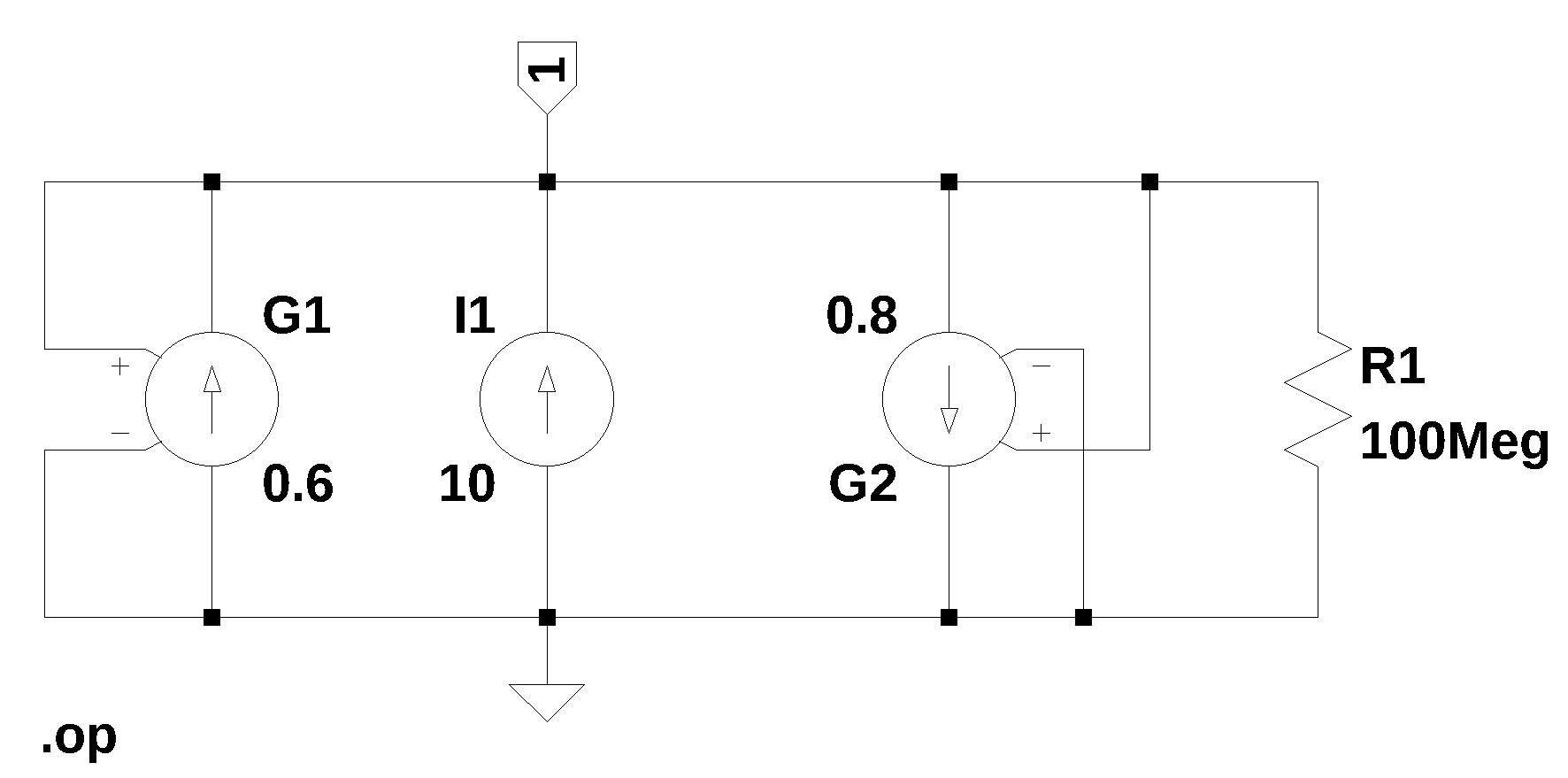
The net list for the circuit was generated by LTSpice and show below:
G1 0 1 1 0 0.6
I1 0 1 10
G2 1 0 1 0 0.8
R1 1 0 100Meg38.1 Load the net list
R1 is commented out.
net_list = '''
G1 0 1 1 0 0.6
I1 0 1 10
G2 1 0 1 0 0.8
*R1 1 0 100e6
'''
38.2 Call the symbolic modified nodal analysis function
report, network_df, i_unk_df, A, X, Z = SymMNA.smna(net_list)Display the equations
# reform X and Z into Matrix type for printing
Xp = Matrix(X)
Zp = Matrix(Z)
temp = ''
for i in range(len(X)):
    temp += '${:s}$<br>'.format(latex(Eq((A*Xp)[i:i+1][0],Zp[i])))

Markdown(temp)
\(v_{1} \left(- g_{1} + g_{2}\right) = I_{1}\)
38.2.1 Netlist statistics
print(report)Net list report
number of lines in netlist: 3
number of branches: 3
number of nodes: 1
number of unknown currents: 0
number of RLC (passive components): 0
number of inductors: 0
number of independent voltage sources: 0
number of independent current sources: 1
number of Op Amps: 0
number of E - VCVS: 0
number of G - VCCS: 2
number of F - CCCS: 0
number of H - CCVS: 0
number of K - Coupled inductors: 0
38.2.2 Connectivity Matrix
A\(\displaystyle \left[\begin{matrix}- g_{1} + g_{2}\end{matrix}\right]\)
38.2.3 Unknown voltages and currents
X\(\displaystyle \left[ v_{1}\right]\)
38.2.4 Known voltages and currents
Z\(\displaystyle \left[ I_{1}\right]\)
38.2.5 Network dataframe
network_df| element | p node | n node | cp node | cn node | Vout | value | Vname | Lname1 | Lname2 | |
|---|---|---|---|---|---|---|---|---|---|---|
| 0 | G1 | 0 | 1 | 1 | 0 | NaN | 0.6 | NaN | NaN | NaN |
| 1 | I1 | 0 | 1 | NaN | NaN | NaN | 10.0 | NaN | NaN | NaN |
| 2 | G2 | 1 | 0 | 1 | 0 | NaN | 0.8 | NaN | NaN | NaN |
38.2.6 Unknown current dataframe
i_unk_df| element | p node | n node |
|---|
38.2.7 Build the network equations
# Put matrices into SymPy
X = Matrix(X)
Z = Matrix(Z)

NE_sym = Eq(A*X,Z)
Turn the free symbols into SymPy variables.
var(str(NE_sym.free_symbols).replace('{','').replace('}',''))\(\displaystyle \left( I_{1}, \ v_{1}, \ g_{2}, \ g_{1}\right)\)
38.3 Symbolic solution
U_sym = solve(NE_sym,X)Display the symbolic solution
temp = ''
for i in U_sym.keys():
    temp += '${:s} = {:s}$<br>'.format(latex(i),latex(U_sym[i]))

Markdown(temp)
\(v_{1} = - \frac{I_{1}}{g_{1} - g_{2}}\)
38.4 Construct a dictionary of element values
element_values = SymMNA.get_part_values(network_df)

# display the component values
for k,v in element_values.items():
    print('{:s} = {:s}'.format(str(k), str(v)))
g1 = 0.6
I1 = 10.0
g2 = 0.838.5 Numerical solution
NE = NE_sym.subs(element_values)Display the equations with numeric values.
temp = ''
for i in range(shape(NE.lhs)[0]):
    temp += '${:s} = {:s}$<br>'.format(latex(NE.rhs[i]),latex(NE.lhs[i]))

Markdown(temp)
\(10.0 = 0.2 v_{1}\)
Solve for voltages and currents.
U = solve(NE,X)Display the numerical solution
Six significant digits are displayed so that results can be compared to LTSpice.
table_header = ['unknown', 'mag']
table_row = []

for name, value in U.items():
    table_row.append([str(name),float(value)])

print(tabulate(table_row, headers=table_header,colalign = ('left','decimal'),tablefmt="simple",floatfmt=('5s','.6f')))
unknown mag
--------- ---------
v1 50.000000The node voltages and current through the sources are solved for. The Sympy generated solution matches the LTSpice results:
--- Operating Point ---V(1): 50 voltage I(I1): 10 device_current I(R1): 5e-07 device_current I(G1): 30 device_current I(G2): 40 device_current
The results from LTSpice agree with the SymPy results.

Find the power absorbed by each source in the circuit.
The results from LTSpice agree with the SymPy results.
element_values[g1]*U[v1]**2 # power through G1\(\displaystyle 1500.0\)
element_values[g2]*U[v1]**2 # power through G2\(\displaystyle 2000.0\)
element_values[I1]*U[v1] # power through I1\(\displaystyle 500.0\)