netlist = '''
R1 2 0 2
C1 0 2 0.5
L1 1 2 3
V1 1 0 1
R2 3 2 1
L2 3 4 1
C2 3 1 0.25
V2 4 0 2
C3 4 3 3
'''Symbolic Modified Nodal Analysis
using Python

Note
- This book is a draft copy and many sections are still under construction.
- Basic spelling and grammar checks have not been completed.
Welcome
Welcome to Symbolic Modified Nodal Analysis using Python. This book is personal project that is being made available online during the development of the book.
The Python code presented in this book will allow students and professionals to automatically generate symbolic network equations from a circuit’s netlist. Then using the power of SymPy, NumPy and SciPy those equations can be symbolically or numerically solved. The JupyterLab notebooks presented in this book can be used as templates to analyze almost any linear electrical circuit.
Quick Example
Consider the schematic shown in Figure 1. This is the type of circuit that you might find as a homework or example problem in an engineering circuit analysis textbook, where the student might be asked to find the steady state voltage at one of the circuit nodes as a function of \(s=j\omega\).
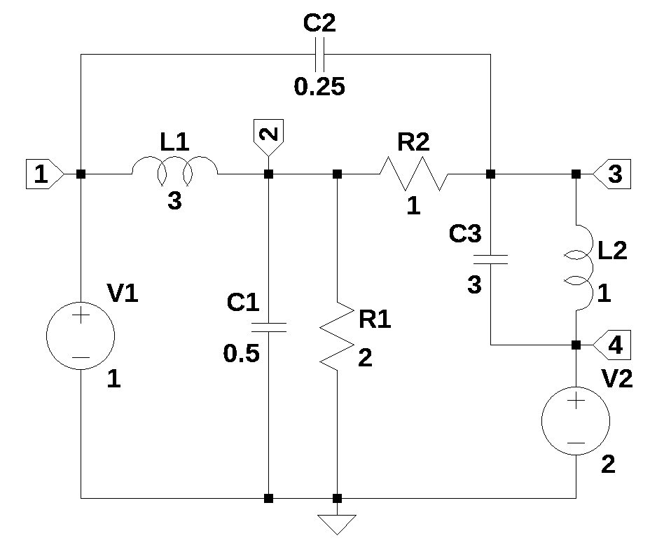
This circuit has two resistors, three capacitors, two inductors and two independent voltage sources. Each of the nodes are labeled along with the reference node. The schematic above was drawn using LTSpice and the netlist was obtained and copied below. The nodes were numbered in no particular order and the reference node is indicated by the ground symbol.
The symbolic modified nodal analysis function, SymMNA.smna(netlist) is called to generate network equations from the netlist.
report, network_df, df2, A, X, Z = SymMNA.smna(netlist)The internals of this function are explained in chapter 4 MNA with Python. Several parameters are returned by the function, but only the matrix \(A\) and vectors \(X\) and \(Z\) are used in this example. The formulation of these parameters are describe in the paragraph, Detailed Structure of the System Matrix. The \(A\) matrix is called the system matrix. The vector \(X\) contains the symbols for the unknown node voltages and the currents. The \(Z\) vector contains the symbols for the newtork Knowns.
The network equations for the circuit can be obtained from the \(A\), \(X\) and \(Z\) parameters returned from the SMNA function and these are formulated into equations and displayed below. Markdown is an IPython function and latex is a SymPy printing function.
# Put matrices into SymPy
X = Matrix(X)
Z = Matrix(Z)

# formulate the network equations
NE_sym = Eq(A*X,Z)

# display the equations with markdown
temp = ''
for i in range(len(X)):
    temp += '${:s}$<br>'.format(latex(Eq((A*X)[i:i+1][0],Z[i])))

Markdown(temp)
\(C_{2} s v_{1} - C_{2} s v_{3} + I_{L1} + I_{V1} = 0\)
\(- I_{L1} + v_{2} \left(C_{1} s + \frac{1}{R_{2}} + \frac{1}{R_{1}}\right) - \frac{v_{3}}{R_{2}} = 0\)
\(- C_{2} s v_{1} - C_{3} s v_{4} + I_{L2} + v_{3} \left(C_{2} s + C_{3} s + \frac{1}{R_{2}}\right) - \frac{v_{2}}{R_{2}} = 0\)
\(- C_{3} s v_{3} + C_{3} s v_{4} - I_{L2} + I_{V2} = 0\)
\(v_{1} = V_{1}\)
\(v_{4} = V_{2}\)
\(- I_{L1} L_{1} s + v_{1} - v_{2} = 0\)
\(- I_{L2} L_{2} s + v_{3} - v_{4} = 0\)
The network equations for the netlist can be solved symbolically using the SymPy function solve and the node voltages and dependent currents are displayed using symbolic notation.
U_sym = solve(NE_sym,X)

temp = ''
for i in U_sym.keys():
    temp += '${:s} = {:s}$<br>'.format(latex(i),latex(U_sym[i]))

Markdown(temp)
\(v_{1} = V_{1}\)
\(v_{2} = \frac{C_{2} L_{1} L_{2} R_{1} V_{1} s^{3} + C_{2} L_{2} R_{1} R_{2} V_{1} s^{2} + C_{3} L_{1} L_{2} R_{1} V_{2} s^{3} + C_{3} L_{2} R_{1} R_{2} V_{1} s^{2} + L_{1} R_{1} V_{2} s + L_{2} R_{1} V_{1} s + R_{1} R_{2} V_{1}}{C_{1} C_{2} L_{1} L_{2} R_{1} R_{2} s^{4} + C_{1} C_{3} L_{1} L_{2} R_{1} R_{2} s^{4} + C_{1} L_{1} L_{2} R_{1} s^{3} + C_{1} L_{1} R_{1} R_{2} s^{2} + C_{2} L_{1} L_{2} R_{1} s^{3} + C_{2} L_{1} L_{2} R_{2} s^{3} + C_{2} L_{2} R_{1} R_{2} s^{2} + C_{3} L_{1} L_{2} R_{1} s^{3} + C_{3} L_{1} L_{2} R_{2} s^{3} + C_{3} L_{2} R_{1} R_{2} s^{2} + L_{1} L_{2} s^{2} + L_{1} R_{1} s + L_{1} R_{2} s + L_{2} R_{1} s + R_{1} R_{2}}\)
\(v_{3} = \frac{C_{1} C_{2} L_{1} L_{2} R_{1} R_{2} V_{1} s^{4} + C_{1} C_{3} L_{1} L_{2} R_{1} R_{2} V_{2} s^{4} + C_{1} L_{1} R_{1} R_{2} V_{2} s^{2} + C_{2} L_{1} L_{2} R_{1} V_{1} s^{3} + C_{2} L_{1} L_{2} R_{2} V_{1} s^{3} + C_{2} L_{2} R_{1} R_{2} V_{1} s^{2} + C_{3} L_{1} L_{2} R_{1} V_{2} s^{3} + C_{3} L_{1} L_{2} R_{2} V_{2} s^{3} + C_{3} L_{2} R_{1} R_{2} V_{2} s^{2} + L_{1} R_{1} V_{2} s + L_{1} R_{2} V_{2} s + L_{2} R_{1} V_{1} s + R_{1} R_{2} V_{2}}{C_{1} C_{2} L_{1} L_{2} R_{1} R_{2} s^{4} + C_{1} C_{3} L_{1} L_{2} R_{1} R_{2} s^{4} + C_{1} L_{1} L_{2} R_{1} s^{3} + C_{1} L_{1} R_{1} R_{2} s^{2} + C_{2} L_{1} L_{2} R_{1} s^{3} + C_{2} L_{1} L_{2} R_{2} s^{3} + C_{2} L_{2} R_{1} R_{2} s^{2} + C_{3} L_{1} L_{2} R_{1} s^{3} + C_{3} L_{1} L_{2} R_{2} s^{3} + C_{3} L_{2} R_{1} R_{2} s^{2} + L_{1} L_{2} s^{2} + L_{1} R_{1} s + L_{1} R_{2} s + L_{2} R_{1} s + R_{1} R_{2}}\)
\(v_{4} = V_{2}\)
\(I_{V1} = \frac{- C_{1} C_{2} C_{3} L_{1} L_{2} R_{1} R_{2} V_{1} s^{5} + C_{1} C_{2} C_{3} L_{1} L_{2} R_{1} R_{2} V_{2} s^{5} - C_{1} C_{2} L_{1} L_{2} R_{1} V_{1} s^{4} - C_{1} C_{2} L_{1} R_{1} R_{2} V_{1} s^{3} + C_{1} C_{2} L_{1} R_{1} R_{2} V_{2} s^{3} - C_{1} C_{2} L_{2} R_{1} R_{2} V_{1} s^{3} - C_{1} C_{3} L_{2} R_{1} R_{2} V_{1} s^{3} - C_{1} L_{2} R_{1} V_{1} s^{2} - C_{1} R_{1} R_{2} V_{1} s - C_{2} C_{3} L_{1} L_{2} R_{1} V_{1} s^{4} + C_{2} C_{3} L_{1} L_{2} R_{1} V_{2} s^{4} - C_{2} C_{3} L_{1} L_{2} R_{2} V_{1} s^{4} + C_{2} C_{3} L_{1} L_{2} R_{2} V_{2} s^{4} - C_{2} C_{3} L_{2} R_{1} R_{2} V_{1} s^{3} + C_{2} C_{3} L_{2} R_{1} R_{2} V_{2} s^{3} - C_{2} L_{1} L_{2} V_{1} s^{3} - C_{2} L_{1} R_{1} V_{1} s^{2} + C_{2} L_{1} R_{1} V_{2} s^{2} - C_{2} L_{1} R_{2} V_{1} s^{2} + C_{2} L_{1} R_{2} V_{2} s^{2} - C_{2} L_{2} R_{2} V_{1} s^{2} - C_{2} R_{1} R_{2} V_{1} s + C_{2} R_{1} R_{2} V_{2} s - C_{3} L_{2} R_{1} V_{1} s^{2} + C_{3} L_{2} R_{1} V_{2} s^{2} - C_{3} L_{2} R_{2} V_{1} s^{2} - L_{2} V_{1} s - R_{1} V_{1} + R_{1} V_{2} - R_{2} V_{1}}{C_{1} C_{2} L_{1} L_{2} R_{1} R_{2} s^{4} + C_{1} C_{3} L_{1} L_{2} R_{1} R_{2} s^{4} + C_{1} L_{1} L_{2} R_{1} s^{3} + C_{1} L_{1} R_{1} R_{2} s^{2} + C_{2} L_{1} L_{2} R_{1} s^{3} + C_{2} L_{1} L_{2} R_{2} s^{3} + C_{2} L_{2} R_{1} R_{2} s^{2} + C_{3} L_{1} L_{2} R_{1} s^{3} + C_{3} L_{1} L_{2} R_{2} s^{3} + C_{3} L_{2} R_{1} R_{2} s^{2} + L_{1} L_{2} s^{2} + L_{1} R_{1} s + L_{1} R_{2} s + L_{2} R_{1} s + R_{1} R_{2}}\)
\(I_{V2} = \frac{C_{1} C_{2} C_{3} L_{1} L_{2} R_{1} R_{2} V_{1} s^{5} - C_{1} C_{2} C_{3} L_{1} L_{2} R_{1} R_{2} V_{2} s^{5} + C_{1} C_{2} L_{1} R_{1} R_{2} V_{1} s^{3} - C_{1} C_{2} L_{1} R_{1} R_{2} V_{2} s^{3} - C_{1} C_{3} L_{1} L_{2} R_{1} V_{2} s^{4} - C_{1} L_{1} R_{1} V_{2} s^{2} + C_{2} C_{3} L_{1} L_{2} R_{1} V_{1} s^{4} - C_{2} C_{3} L_{1} L_{2} R_{1} V_{2} s^{4} + C_{2} C_{3} L_{1} L_{2} R_{2} V_{1} s^{4} - C_{2} C_{3} L_{1} L_{2} R_{2} V_{2} s^{4} + C_{2} C_{3} L_{2} R_{1} R_{2} V_{1} s^{3} - C_{2} C_{3} L_{2} R_{1} R_{2} V_{2} s^{3} + C_{2} L_{1} R_{1} V_{1} s^{2} - C_{2} L_{1} R_{1} V_{2} s^{2} + C_{2} L_{1} R_{2} V_{1} s^{2} - C_{2} L_{1} R_{2} V_{2} s^{2} + C_{2} R_{1} R_{2} V_{1} s - C_{2} R_{1} R_{2} V_{2} s - C_{3} L_{1} L_{2} V_{2} s^{3} + C_{3} L_{2} R_{1} V_{1} s^{2} - C_{3} L_{2} R_{1} V_{2} s^{2} - L_{1} V_{2} s + R_{1} V_{1} - R_{1} V_{2}}{C_{1} C_{2} L_{1} L_{2} R_{1} R_{2} s^{4} + C_{1} C_{3} L_{1} L_{2} R_{1} R_{2} s^{4} + C_{1} L_{1} L_{2} R_{1} s^{3} + C_{1} L_{1} R_{1} R_{2} s^{2} + C_{2} L_{1} L_{2} R_{1} s^{3} + C_{2} L_{1} L_{2} R_{2} s^{3} + C_{2} L_{2} R_{1} R_{2} s^{2} + C_{3} L_{1} L_{2} R_{1} s^{3} + C_{3} L_{1} L_{2} R_{2} s^{3} + C_{3} L_{2} R_{1} R_{2} s^{2} + L_{1} L_{2} s^{2} + L_{1} R_{1} s + L_{1} R_{2} s + L_{2} R_{1} s + R_{1} R_{2}}\)
\(I_{L1} = \frac{C_{1} C_{2} L_{2} R_{1} R_{2} V_{1} s^{3} + C_{1} C_{3} L_{2} R_{1} R_{2} V_{1} s^{3} + C_{1} L_{2} R_{1} V_{1} s^{2} + C_{1} R_{1} R_{2} V_{1} s + C_{2} L_{2} R_{2} V_{1} s^{2} + C_{3} L_{2} R_{1} V_{1} s^{2} - C_{3} L_{2} R_{1} V_{2} s^{2} + C_{3} L_{2} R_{2} V_{1} s^{2} + L_{2} V_{1} s + R_{1} V_{1} - R_{1} V_{2} + R_{2} V_{1}}{C_{1} C_{2} L_{1} L_{2} R_{1} R_{2} s^{4} + C_{1} C_{3} L_{1} L_{2} R_{1} R_{2} s^{4} + C_{1} L_{1} L_{2} R_{1} s^{3} + C_{1} L_{1} R_{1} R_{2} s^{2} + C_{2} L_{1} L_{2} R_{1} s^{3} + C_{2} L_{1} L_{2} R_{2} s^{3} + C_{2} L_{2} R_{1} R_{2} s^{2} + C_{3} L_{1} L_{2} R_{1} s^{3} + C_{3} L_{1} L_{2} R_{2} s^{3} + C_{3} L_{2} R_{1} R_{2} s^{2} + L_{1} L_{2} s^{2} + L_{1} R_{1} s + L_{1} R_{2} s + L_{2} R_{1} s + R_{1} R_{2}}\)
\(I_{L2} = \frac{C_{1} C_{2} L_{1} R_{1} R_{2} V_{1} s^{3} - C_{1} C_{2} L_{1} R_{1} R_{2} V_{2} s^{3} - C_{1} L_{1} R_{1} V_{2} s^{2} + C_{2} L_{1} R_{1} V_{1} s^{2} - C_{2} L_{1} R_{1} V_{2} s^{2} + C_{2} L_{1} R_{2} V_{1} s^{2} - C_{2} L_{1} R_{2} V_{2} s^{2} + C_{2} R_{1} R_{2} V_{1} s - C_{2} R_{1} R_{2} V_{2} s - L_{1} V_{2} s + R_{1} V_{1} - R_{1} V_{2}}{C_{1} C_{2} L_{1} L_{2} R_{1} R_{2} s^{4} + C_{1} C_{3} L_{1} L_{2} R_{1} R_{2} s^{4} + C_{1} L_{1} L_{2} R_{1} s^{3} + C_{1} L_{1} R_{1} R_{2} s^{2} + C_{2} L_{1} L_{2} R_{1} s^{3} + C_{2} L_{1} L_{2} R_{2} s^{3} + C_{2} L_{2} R_{1} R_{2} s^{2} + C_{3} L_{1} L_{2} R_{1} s^{3} + C_{3} L_{1} L_{2} R_{2} s^{3} + C_{3} L_{2} R_{1} R_{2} s^{2} + L_{1} L_{2} s^{2} + L_{1} R_{1} s + L_{1} R_{2} s + L_{2} R_{1} s + R_{1} R_{2}}\)
As you can see in this example, generating a set of network equations from a schematic’s netlist is rather easy with the help of Python. Then SymPy can be used to solve the network equations, if the system of equations is not too large. The symbolic solutions for the node voltages and unknown currents in this example have rather long expressions. The slider bar can be used to view the expressions which extend beyond the margins of the book’s page. Generating and solving the network equations took less than one second on my i3 desktop computer. Numerical values can be substituted for the symbolic values and NumPy can used to obtain a solution, even for relatively large networks.
Colophon
This book was written in R MarkDown using plain text files and JupyterLab notebooks. The source files were rendered into an HTML book using Quarto, an open-source scientific and technical publishing system. HTML books are actually just a special type of Quarto Website. Quarto does a good job of formatting the documents into web pages for a book. Some of the lines of code and mathematical expressions are wider than the page and Quarto inserts a slider bar in the code or equation windows. Chapter and paragraph numbering are automatically generated by Quarto as well as the numbering of figures and tables.
I don’t have a proof reader or professional editors for this project. Instead, I’m relying on the LibreOffice spell checker and the grammar and spell checker of Google Docs to help me with the proof reading part of the writing process. Employing professional editors to work on this project may happen in the future.
Some sections of this work were developed with the assistance of Gemini, an artificial intelligence developed by Google. While this technology was utilized to draft some of the initial content, second and subsequent draft versions have been meticulously reviewed by the author. Every Gemini assisted section has been reworded for style and fact-checked for accuracy.
Python code contained in this book can run in a browser-based environment, see Appendix C — Google Colab. Additionally, online schematics editors are available, see Appendix E — EasyEDA. By using web based tools, the reader is not required to install any programs.
Source Code
Archived source code for this project can be found on GitHub. Here you will find markdown files, JupyterLab notebooks, LTSpice schematics and image files. I will do my best to keep these files current. All the source code is subject to the license stated in License.
Overview
The first four chapters introduce the topic of circuit analysis with some light background theory and describe my implementation of symbolic modified nodal analysis with Python. In addition, basic circuit analysis topics of - Resistive Networks, RLC Networks, Transfer Function, Transient Analysis, Mutual Inductance and Initial Conditions using Python are presented.
The next part of the book, Example Problems, contains circuit analysis example problems. This is followed by Validation Tests, which are 15 test circuits used to validate the Python code. This is followed by the Appendices which contain: references, code listing, notes about Colab and EasyEDA, a change log and a short history of electric circuit analysis.
The right margin of each page contains index with links to all the chapters. The left margin contains links to sections within the current chapter.
Feedback
If you have complaints, find any errors, or have suggestions, send me an email at:
juan1543cabrillo@sudomail.com
Citation
If you find the book useful, please cite it as follows:
@online{Tiburonboy2024,
    author = {Tiburonboy},
    title = {Symbolic Modified Nodal Analysis using Python},
    year = {2024},
    url = {https://tiburonboy.github.io/Symbolic-Modified-Nodal-Analysis-using-Python/},
    urldate = {2025-08-13}
}
Python Module Versions
The following versions were used in this book.
The Jupyter notebooks are available from my GitHub repository. The results presented in this book should be reproducible if the libraries and modules have the same version numbers.
Revision History
This book will be updated occasionally to update content and fix spelling and grammar mistakes - see Table B.2. Additionally, new content will be added as new chapters in the Example Problems section. The published date at the top of this page is the date of last revision.
License
This work (includes python code, documentation, test circuits, etc.) is licensed under a Creative Commons Attribution-ShareAlike 4.0 International License.
- Share — Copy and redistribute the material in any medium or format.
- Adapt — Remix, transform, and build upon the material for any purpose, even commercially.
- Attribution — You must give appropriate credit, provide a link to the license, and indicate if changes were made. You may do so in any reasonable manner, but not in any way that suggests the licensor endorses you or your use.
- ShareAlike — If you remix, transform, or build upon the material, you must distribute your contributions under the same license as the original.
