#import os
from sympy import *
import numpy as np
from tabulate import tabulate
from scipy import signal
import matplotlib.pyplot as plt
import pandas as pd
import SymMNA
from IPython.display import display, Markdown, Math, Latex
init_printing()32 Test 3
The circuit in Figure 32.1 is from Johnson, Hilburn, and Johnson (1978) (Figure 4.8), but modified to include a capactior and inductor. AC analysis was performed at 1 rad/sec and also over a range of frequencies. The results are compared to those obtained from LTSpice.
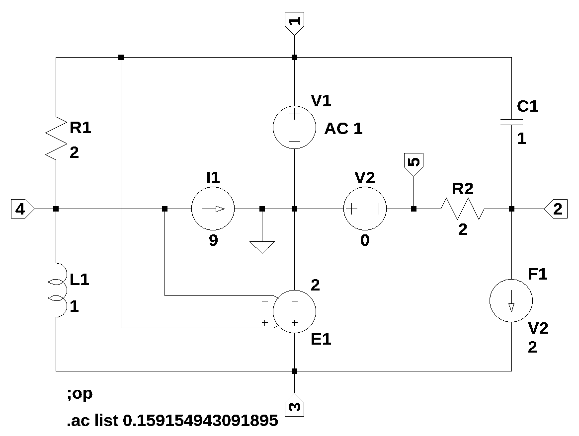
The net list for Figure 32.1 was generated by LTSpice and show below:
R2 2 5 2
V1 1 0 0 AC 1
I1 4 0 9
V2 0 5 0
E1 3 0 1 4 2
F1 2 3 V2 2
R1 1 4 2
C1 1 2 1
L1 4 3 132.1 Load the net list
net_list = '''
R2 2 5 2
V1 1 0 1
I1 4 0 9
V2 0 5 0
E1 3 0 1 4 2
F1 2 3 V2 2
R1 1 4 2
C1 1 2 1
L1 4 3 1
'''
32.2 Call the symbolic modified nodal analysis function
report, network_df, i_unk_df, A, X, Z = SymMNA.smna(net_list)Display the equations
# reform X and Z into Matrix type for printing
Xp = Matrix(X)
Zp = Matrix(Z)
temp = ''
for i in range(len(X)):
    temp += '${:s}$<br>'.format(latex(Eq((A*Xp)[i:i+1][0],Zp[i])))

Markdown(temp)
\(- C_{1} s v_{2} + I_{V1} + v_{1} \left(C_{1} s + \frac{1}{R_{1}}\right) - \frac{v_{4}}{R_{1}} = 0\)
\(- C_{1} s v_{1} + I_{F1} + v_{2} \left(C_{1} s + \frac{1}{R_{2}}\right) - \frac{v_{5}}{R_{2}} = 0\)
\(I_{Ea1} - I_{F1} - I_{L1} = 0\)
\(I_{L1} - \frac{v_{1}}{R_{1}} + \frac{v_{4}}{R_{1}} = - I_{1}\)
\(- I_{V2} - \frac{v_{2}}{R_{2}} + \frac{v_{5}}{R_{2}} = 0\)
\(v_{1} = V_{1}\)
\(- v_{5} = V_{2}\)
\(- ea_{1} v_{1} + ea_{1} v_{4} + v_{3} = 0\)
\(I_{F1} - I_{V2} f_{1} = 0\)
\(- I_{L1} L_{1} s - v_{3} + v_{4} = 0\)
32.2.1 Netlist statistics
print(report)Net list report
number of lines in netlist: 9
number of branches: 9
number of nodes: 5
number of unknown currents: 5
number of RLC (passive components): 4
number of inductors: 1
number of independent voltage sources: 2
number of independent current sources: 1
number of Op Amps: 0
number of E - VCVS: 1
number of G - VCCS: 0
number of F - CCCS: 1
number of H - CCVS: 0
number of K - Coupled inductors: 0
32.2.2 Connectivity Matrix
A\(\displaystyle \left[\begin{matrix}C_{1} s + \frac{1}{R_{1}} & - C_{1} s & 0 & - \frac{1}{R_{1}} & 0 & 1 & 0 & 0 & 0 & 0\\- C_{1} s & C_{1} s + \frac{1}{R_{2}} & 0 & 0 & - \frac{1}{R_{2}} & 0 & 0 & 0 & 1 & 0\\0 & 0 & 0 & 0 & 0 & 0 & 0 & 1 & -1 & -1\\- \frac{1}{R_{1}} & 0 & 0 & \frac{1}{R_{1}} & 0 & 0 & 0 & 0 & 0 & 1\\0 & - \frac{1}{R_{2}} & 0 & 0 & \frac{1}{R_{2}} & 0 & -1 & 0 & 0 & 0\\1 & 0 & 0 & 0 & 0 & 0 & 0 & 0 & 0 & 0\\0 & 0 & 0 & 0 & -1 & 0 & 0 & 0 & 0 & 0\\- ea_{1} & 0 & 1 & ea_{1} & 0 & 0 & 0 & 0 & 0 & 0\\0 & 0 & 0 & 0 & 0 & 0 & - f_{1} & 0 & 1 & 0\\0 & 0 & -1 & 1 & 0 & 0 & 0 & 0 & 0 & - L_{1} s\end{matrix}\right]\)
32.2.3 Unknown voltages and currents
X\(\displaystyle \left[ v_{1}, \ v_{2}, \ v_{3}, \ v_{4}, \ v_{5}, \ I_{V1}, \ I_{V2}, \ I_{Ea1}, \ I_{F1}, \ I_{L1}\right]\)
32.2.4 Known voltages and currents
Z\(\displaystyle \left[ 0, \ 0, \ 0, \ - I_{1}, \ 0, \ V_{1}, \ V_{2}, \ 0, \ 0, \ 0\right]\)
32.2.5 Network dataframe
network_df| element | p node | n node | cp node | cn node | Vout | value | Vname | Lname1 | Lname2 | |
|---|---|---|---|---|---|---|---|---|---|---|
| 0 | V1 | 1 | 0 | NaN | NaN | NaN | 1.0 | NaN | NaN | NaN |
| 1 | V2 | 0 | 5 | NaN | NaN | NaN | 0.0 | NaN | NaN | NaN |
| 2 | R2 | 2 | 5 | NaN | NaN | NaN | 2.0 | NaN | NaN | NaN |
| 3 | I1 | 4 | 0 | NaN | NaN | NaN | 9.0 | NaN | NaN | NaN |
| 4 | Ea1 | 3 | 0 | 1 | 4 | NaN | 2.0 | NaN | NaN | NaN |
| 5 | F1 | 2 | 3 | NaN | NaN | NaN | 2.0 | V2 | NaN | NaN |
| 6 | R1 | 1 | 4 | NaN | NaN | NaN | 2.0 | NaN | NaN | NaN |
| 7 | C1 | 1 | 2 | NaN | NaN | NaN | 1.0 | NaN | NaN | NaN |
| 8 | L1 | 4 | 3 | NaN | NaN | NaN | 1.0 | NaN | NaN | NaN |
32.2.6 Unknown current dataframe
i_unk_df| element | p node | n node | |
|---|---|---|---|
| 0 | V1 | 1 | 0 |
| 1 | V2 | 0 | 5 |
| 2 | Ea1 | 3 | 0 |
| 3 | F1 | 2 | 3 |
| 4 | L1 | 4 | 3 |
32.2.7 Build the network equations
# Put matrices into SymPy
X = Matrix(X)
Z = Matrix(Z)

NE_sym = Eq(A*X,Z)
Turn the free symbols into SymPy variables.
var(str(NE_sym.free_symbols).replace('{','').replace('}',''))\(\displaystyle \left( C_{1}, \ R_{1}, \ v_{4}, \ I_{V2}, \ V_{1}, \ I_{1}, \ L_{1}, \ I_{Ea1}, \ v_{1}, \ v_{3}, \ ea_{1}, \ s, \ f_{1}, \ V_{2}, \ v_{5}, \ I_{F1}, \ I_{V1}, \ v_{2}, \ R_{2}, \ I_{L1}\right)\)
32.3 Symbolic solution
U_sym = solve(NE_sym,X)Display the symbolic solution
temp = ''
for i in U_sym.keys():
    temp += '${:s} = {:s}$<br>'.format(latex(i),latex(U_sym[i]))

Markdown(temp)
\(v_{1} = V_{1}\)
\(v_{2} = \frac{C_{1} R_{2} V_{1} s + V_{2} f_{1} - V_{2}}{C_{1} R_{2} s - f_{1} + 1}\)
\(v_{3} = \frac{I_{1} L_{1} R_{1} ea_{1} s + R_{1} V_{1} ea_{1}}{L_{1} s + R_{1} ea_{1} + R_{1}}\)
\(v_{4} = \frac{- I_{1} L_{1} R_{1} s + L_{1} V_{1} s + R_{1} V_{1} ea_{1}}{L_{1} s + R_{1} ea_{1} + R_{1}}\)
\(v_{5} = - V_{2}\)
\(I_{V1} = \frac{- C_{1} I_{1} L_{1} R_{2} s^{2} + C_{1} L_{1} V_{1} f_{1} s^{2} - C_{1} L_{1} V_{1} s^{2} + C_{1} L_{1} V_{2} f_{1} s^{2} - C_{1} L_{1} V_{2} s^{2} + C_{1} R_{1} V_{1} ea_{1} f_{1} s - C_{1} R_{1} V_{1} ea_{1} s + C_{1} R_{1} V_{1} f_{1} s - C_{1} R_{1} V_{1} s + C_{1} R_{1} V_{2} ea_{1} f_{1} s - C_{1} R_{1} V_{2} ea_{1} s + C_{1} R_{1} V_{2} f_{1} s - C_{1} R_{1} V_{2} s - C_{1} R_{2} V_{1} s + I_{1} L_{1} f_{1} s - I_{1} L_{1} s + V_{1} f_{1} - V_{1}}{C_{1} L_{1} R_{2} s^{2} + C_{1} R_{1} R_{2} ea_{1} s + C_{1} R_{1} R_{2} s - L_{1} f_{1} s + L_{1} s - R_{1} ea_{1} f_{1} + R_{1} ea_{1} - R_{1} f_{1} + R_{1}}\)
\(I_{V2} = \frac{- C_{1} V_{1} s - C_{1} V_{2} s}{C_{1} R_{2} s - f_{1} + 1}\)
\(I_{Ea1} = \frac{- C_{1} I_{1} R_{1} R_{2} ea_{1} s - C_{1} I_{1} R_{1} R_{2} s - C_{1} L_{1} V_{1} f_{1} s^{2} - C_{1} L_{1} V_{2} f_{1} s^{2} - C_{1} R_{1} V_{1} ea_{1} f_{1} s - C_{1} R_{1} V_{1} f_{1} s - C_{1} R_{1} V_{2} ea_{1} f_{1} s - C_{1} R_{1} V_{2} f_{1} s + C_{1} R_{2} V_{1} s + I_{1} R_{1} ea_{1} f_{1} - I_{1} R_{1} ea_{1} + I_{1} R_{1} f_{1} - I_{1} R_{1} - V_{1} f_{1} + V_{1}}{C_{1} L_{1} R_{2} s^{2} + C_{1} R_{1} R_{2} ea_{1} s + C_{1} R_{1} R_{2} s - L_{1} f_{1} s + L_{1} s - R_{1} ea_{1} f_{1} + R_{1} ea_{1} - R_{1} f_{1} + R_{1}}\)
\(I_{F1} = \frac{- C_{1} V_{1} f_{1} s - C_{1} V_{2} f_{1} s}{C_{1} R_{2} s - f_{1} + 1}\)
\(I_{L1} = \frac{- I_{1} R_{1} ea_{1} - I_{1} R_{1} + V_{1}}{L_{1} s + R_{1} ea_{1} + R_{1}}\)
32.4 Construct a dictionary of element values
element_values = SymMNA.get_part_values(network_df)

# display the component values
for k,v in element_values.items():
    print('{:s} = {:s}'.format(str(k), str(v)))
V1 = 1.0
V2 = 0.0
R2 = 2.0
I1 = 9.0
ea1 = 2.0
f1 = 2.0
R1 = 2.0
C1 = 1.0
L1 = 1.032.5 DC operating point
Both V1 and I1 are active.
NE = NE_sym.subs(element_values)
NE_dc = NE.subs({s:0})
Display the equations with numeric values.
temp = ''
for i in range(shape(NE_dc.lhs)[0]):
    temp += '${:s} = {:s}$<br>'.format(latex(NE_dc.rhs[i]),latex(NE_dc.lhs[i]))

Markdown(temp)
\(0 = I_{V1} + 0.5 v_{1} - 0.5 v_{4}\)
\(0 = I_{F1} + 0.5 v_{2} - 0.5 v_{5}\)
\(0 = I_{Ea1} - I_{F1} - I_{L1}\)
\(-9.0 = I_{L1} - 0.5 v_{1} + 0.5 v_{4}\)
\(0 = - I_{V2} - 0.5 v_{2} + 0.5 v_{5}\)
\(1.0 = v_{1}\)
\(0 = - v_{5}\)
\(0 = - 2.0 v_{1} + v_{3} + 2.0 v_{4}\)
\(0 = I_{F1} - 2.0 I_{V2}\)
\(0 = - v_{3} + v_{4}\)
Solve for voltages and currents.
U_dc = solve(NE_dc,X)Display the numerical solution
Six significant digits are displayed so that results can be compared to LTSpice.
table_header = ['unknown', 'mag']
table_row = []

for name, value in U_dc.items():
    table_row.append([str(name),float(value)])

print(tabulate(table_row, headers=table_header,colalign = ('left','decimal'),tablefmt="simple",floatfmt=('5s','.6f')))
unknown mag
--------- ---------
v1 1.000000
v2 0.000000
v3 0.666667
v4 0.666667
v5 0.000000
I_V1 -0.166667
I_V2 0.000000
I_Ea1 -8.833333
I_F1 0.000000
I_L1 -8.833333The node voltages and current through the sources are solved for. The Sympy generated solution matches the LTSpice results:
       --- Operating Point ---

V(2):    -2e-12  voltage
V(5):    0   voltage
V(1):    1   voltage
V(4):    0.666667    voltage
V(3):    0.666667    voltage
I(C1):   1e-12   device_current
I(F1):   2e-12   device_current
I(L1):   -8.83333    device_current
I(I1):   9   device_current
I(R2):   -1e-12  device_current
I(R1):   0.166667    device_current
I(E1):   -8.83333    device_current
I(V1):   -0.166667   device_current
I(V2):   1e-12   device_current
The results from LTSpice agree with the SymPy results.
32.5.1 AC analysis
Solve equations for \(\omega\) equal to 1 radian per second, s = 1j.
Need to set I1 = 0
element_values[I1] = 0
NE = NE_sym.subs(element_values)
NE_w1 = NE.subs({s:1j})
Display the equations with numeric values.
temp = ''
for i in range(shape(NE_w1.lhs)[0]):
    temp += '${:s} = {:s}$<br>'.format(latex(NE_w1.rhs[i]),latex(NE_w1.lhs[i]))

Markdown(temp)
\(0 = I_{V1} + v_{1} \cdot \left(0.5 + 1.0 i\right) - 1.0 i v_{2} - 0.5 v_{4}\)
\(0 = I_{F1} - 1.0 i v_{1} + v_{2} \cdot \left(0.5 + 1.0 i\right) - 0.5 v_{5}\)
\(0 = I_{Ea1} - I_{F1} - I_{L1}\)
\(0 = I_{L1} - 0.5 v_{1} + 0.5 v_{4}\)
\(0 = - I_{V2} - 0.5 v_{2} + 0.5 v_{5}\)
\(1.0 = v_{1}\)
\(0 = - v_{5}\)
\(0 = - 2.0 v_{1} + v_{3} + 2.0 v_{4}\)
\(0 = I_{F1} - 2.0 I_{V2}\)
\(0 = - 1.0 i I_{L1} - v_{3} + v_{4}\)
Solve for voltages and currents.
U_w1 = solve(NE_w1,X)Display the numerical solution
Six significant digits are displayed so that results can be compared to LTSpice.
table_header = ['unknown', 'mag','phase, deg']
table_row = []

for name, value in U_w1.items():
    table_row.append([str(name),float(abs(value)),float(arg(value)*180/np.pi)])

print(tabulate(table_row, headers=table_header,colalign = ('left','decimal','decimal'),tablefmt="simple",floatfmt=('5s','.6f','.6f')))
unknown mag phase, deg
--------- -------- ------------
v1 1.000000 0.000000
v2 0.894427 -26.565051
v3 0.657596 -9.462322
v4 0.677834 4.573921
v5 0.000000 nan
I_V1 0.294086 -36.027373
I_V2 0.447214 153.434949
I_Ea1 0.738882 149.683220
I_F1 0.894427 153.434949
I_L1 0.164399 -9.462322The LTSpice solution is shown below:
       --- AC Analysis ---

frequency:  0.159155    Hz
V(2):   mag:   0.894427 phase:   -26.5651°  voltage
V(5):   mag:          0 phase:          0°  voltage
V(1):   mag:          1 phase:          0°  voltage
V(4):   mag:   0.677834 phase:    4.57392°  voltage
V(3):   mag:   0.657596 phase:   -9.46232°  voltage
I(C1):  mag:   0.447214 phase:    153.435°  device_current
I(F1):  mag:   0.894427 phase:    153.435°  device_current
I(L1):  mag:   0.164399 phase:   -9.46232°  device_current
I(I1):  mag:          0 phase:          0°  device_current
I(R2):  mag:   0.447214 phase:   -26.5651°  device_current
I(R1):  mag:   0.164399 phase:   -9.46232°  device_current
I(E1):  mag:   0.738882 phase:    149.683°  device_current
I(V1):  mag:   0.294086 phase:   -36.0274°  device_current
I(V2):  mag:   0.447214 phase:    153.435°  device_current
32.5.2 AC Sweep
Looking at node 2 voltage and comparing the results with those obtained from LTSpice. Thr frequenct weep is from 0.01 Hz to 1 Hz.
NE = NE_sym.subs(element_values)Display the equations with numeric values.
temp = ''
for i in range(shape(NE.lhs)[0]):
    temp += '${:s} = {:s}$<br>'.format(latex(NE.rhs[i]),latex(NE.lhs[i]))

Markdown(temp)
\(0 = I_{V1} - 1.0 s v_{2} + v_{1} \cdot \left(1.0 s + 0.5\right) - 0.5 v_{4}\)
\(0 = I_{F1} - 1.0 s v_{1} + v_{2} \cdot \left(1.0 s + 0.5\right) - 0.5 v_{5}\)
\(0 = I_{Ea1} - I_{F1} - I_{L1}\)
\(0 = I_{L1} - 0.5 v_{1} + 0.5 v_{4}\)
\(0 = - I_{V2} - 0.5 v_{2} + 0.5 v_{5}\)
\(1.0 = v_{1}\)
\(0 = - v_{5}\)
\(0 = - 2.0 v_{1} + v_{3} + 2.0 v_{4}\)
\(0 = I_{F1} - 2.0 I_{V2}\)
\(0 = - 1.0 I_{L1} s - v_{3} + v_{4}\)
Solve for voltages and currents.
U_ac = solve(NE,X)32.5.3 Plot the voltage at node 2
H = U_ac[v2]num, denom = fraction(H) #returns numerator and denominator
# convert symbolic to numpy polynomial
a = np.array(Poly(num, s).all_coeffs(), dtype=float)
b = np.array(Poly(denom, s).all_coeffs(), dtype=float)
system = (a, b)#x = np.linspace(0.01*2*np.pi, 1*2*np.pi, 200, endpoint=True)
x = np.logspace(-2, 0, 200, endpoint=False)*2*np.pi
w, mag, phase = signal.bode(system, w=x) # returns: rad/s, mag in dB, phase in degLoad the csv file of node 2 voltage over the sweep range and plot along with the results obtained from SymPy.
fn = 'test_3.csv' # data from LTSpice
LTSpice_data = np.genfromtxt(fn, delimiter=',')
# initaliaze some empty arrays
frequency = np.zeros(len(LTSpice_data))
voltage = np.zeros(len(LTSpice_data)).astype(complex)
# convert the csv data to complex numbers and store in the array
for i in range(len(LTSpice_data)):
frequency[i] = LTSpice_data[i][0]
voltage[i] = LTSpice_data[i][1] + LTSpice_data[i][2]*1jfig, ax1 = plt.subplots()
ax1.set_ylabel('magnitude, dB')
ax1.set_xlabel('frequency, Hz')
plt.semilogx(frequency, 20*np.log10(np.abs(voltage)),'-r') # Bode magnitude plot
plt.semilogx(w/(2*np.pi), mag,'-b') # Bode magnitude plot
ax1.tick_params(axis='y')
ax1.set_ylim((-30,20))
plt.grid()
# instantiate a second y-axes that shares the same x-axis
ax2 = ax1.twinx()
color = 'tab:blue'
plt.semilogx(frequency, np.angle(voltage)*180/np.pi,':',color=color) # Bode phase plot
plt.semilogx(w/(2*np.pi), phase,':',color='tab:red') # Bode phase plot
ax2.set_ylabel('phase, deg',color=color)
ax2.tick_params(axis='y', labelcolor=color)
#ax2.set_ylim((-5,25))
plt.title('Magnitude and phase response')
plt.show()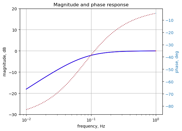
fig, ax1 = plt.subplots()
ax1.set_ylabel('magnitude difference')
ax1.set_xlabel('frequency, Hz')

plt.semilogx(frequency[0:-1], np.abs(voltage[0:-1])-10**(mag/20),'-r')    # Bode magnitude plot
#plt.semilogx(w/(2*np.pi), mag,'-b')    # Bode magnitude plot

ax1.tick_params(axis='y')
#ax1.set_ylim((-30,20))
plt.grid()

# instantiate a second y-axes that shares the same x-axis
ax2 = ax1.twinx()
color = 'tab:blue'

plt.semilogx(frequency[0:-1], np.unwrap(2*np.angle(voltage[0:-1])/2) *180/np.pi - phase,':',color=color)  # Bode phase plot
#plt.semilogx(w/(2*np.pi), phase,':',color='tab:red')  # Bode phase plot

ax2.set_ylabel('phase difference, deg',color=color)
ax2.tick_params(axis='y', labelcolor=color)
#ax2.set_ylim((-5,25))

plt.title('Difference between LTSpice and Python results')
plt.show()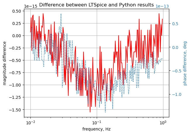
The SymPy and LTSpice results overlay each other. The scale for the magnitude is \(10^{-15}\) and \(10^{-13}\) for the phase indicating the numerical difference is very small.