from sympy import *
import numpy as np
from tabulate import tabulate
from scipy import signal
import matplotlib.pyplot as plt
import pandas as pd
import SymMNA
from IPython.display import display, Markdown, Math, Latex
init_printing()30 Test 1
The circuit in Figure 30.1 is from Johnson, Hilburn, and Johnson (1978) (Figure 4.8). The circuit has five nodes and nine branches. There are two independent voltage sources, V1 and V2. The value of V2 is 0 volts and the current through V2 is needed for F1, the current controlled current source. There is one independent current source, I1. E1 is a voltage controlled voltage source. The circuit contains four resistors.
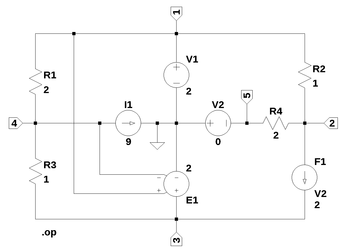
The netlist for Figure 30.1 was generated by LTSpice and show below:
R2 1 2 1
R3 4 3 1
R4 2 5 2
V1 1 0 2
I1 4 0 9
V2 0 5 0
E1 3 0 1 4 2
F1 2 3 V2 2
R1 1 4 2
The following Python modules are used in this notebook.
30.1 Load the netlist
The netlist for the circuit is pasted into the code cell below. In Python a triple-quoted string includes whitespace, tabs and newlines. The newlines characters are needed to mark the end of each SPICE statement in the netlist.
net_list = '''
R2 1 2 1
R3 4 3 1
R4 2 5 2
V1 1 0 2
I1 4 0 9
V2 0 5 0
E1 3 0 1 4 2
F1 2 3 V2 2
R1 1 4 2
'''
30.2 Call the symbolic modified nodal analysis function
report, network_df, i_unk_df, A, X, Z = SymMNA.smna(net_list)The network equations for the circuit can be obtained from the A, X and Z values returned from the SMNA function. The A, X and Z are formulated into equations and displayed below. Markdown is an IPython function and latex is a SymPy printing function.
# reform X and Z into Matrix type for printing
Xp = Matrix(X)
Zp = Matrix(Z)
temp = ''
for i in range(len(X)):
    temp += '${:s}$<br>'.format(latex(Eq((A*Xp)[i:i+1][0],Zp[i])))

Markdown(temp)
\(I_{V1} + v_{1} \cdot \left(\frac{1}{R_{2}} + \frac{1}{R_{1}}\right) - \frac{v_{2}}{R_{2}} - \frac{v_{4}}{R_{1}} = 0\)
\(I_{F1} + v_{2} \cdot \left(\frac{1}{R_{4}} + \frac{1}{R_{2}}\right) - \frac{v_{5}}{R_{4}} - \frac{v_{1}}{R_{2}} = 0\)
\(I_{Ea1} - I_{F1} + \frac{v_{3}}{R_{3}} - \frac{v_{4}}{R_{3}} = 0\)
\(v_{4} \cdot \left(\frac{1}{R_{3}} + \frac{1}{R_{1}}\right) - \frac{v_{3}}{R_{3}} - \frac{v_{1}}{R_{1}} = - I_{1}\)
\(- I_{V2} - \frac{v_{2}}{R_{4}} + \frac{v_{5}}{R_{4}} = 0\)
\(v_{1} = V_{1}\)
\(- v_{5} = V_{2}\)
\(- ea_{1} v_{1} + ea_{1} v_{4} + v_{3} = 0\)
\(I_{F1} - I_{V2} f_{1} = 0\)
30.2.1 Netlist statistics
print(report)Net list report
number of lines in netlist: 9
number of branches: 9
number of nodes: 5
number of unknown currents: 4
number of RLC (passive components): 4
number of inductors: 0
number of independent voltage sources: 2
number of independent current sources: 1
number of Op Amps: 0
number of E - VCVS: 1
number of G - VCCS: 0
number of F - CCCS: 1
number of H - CCVS: 0
number of K - Coupled inductors: 0
30.2.2 Connectivity Matrix
A\(\displaystyle \left[\begin{matrix}\frac{1}{R_{2}} + \frac{1}{R_{1}} & - \frac{1}{R_{2}} & 0 & - \frac{1}{R_{1}} & 0 & 1 & 0 & 0 & 0\\- \frac{1}{R_{2}} & \frac{1}{R_{4}} + \frac{1}{R_{2}} & 0 & 0 & - \frac{1}{R_{4}} & 0 & 0 & 0 & 1\\0 & 0 & \frac{1}{R_{3}} & - \frac{1}{R_{3}} & 0 & 0 & 0 & 1 & -1\\- \frac{1}{R_{1}} & 0 & - \frac{1}{R_{3}} & \frac{1}{R_{3}} + \frac{1}{R_{1}} & 0 & 0 & 0 & 0 & 0\\0 & - \frac{1}{R_{4}} & 0 & 0 & \frac{1}{R_{4}} & 0 & -1 & 0 & 0\\1 & 0 & 0 & 0 & 0 & 0 & 0 & 0 & 0\\0 & 0 & 0 & 0 & -1 & 0 & 0 & 0 & 0\\- ea_{1} & 0 & 1 & ea_{1} & 0 & 0 & 0 & 0 & 0\\0 & 0 & 0 & 0 & 0 & 0 & - f_{1} & 0 & 1\end{matrix}\right]\)
30.2.3 Unknown voltages and currents
X\(\displaystyle \left[ v_{1}, \ v_{2}, \ v_{3}, \ v_{4}, \ v_{5}, \ I_{V1}, \ I_{V2}, \ I_{Ea1}, \ I_{F1}\right]\)
30.2.4 Known voltages and currents
Z\(\displaystyle \left[ 0, \ 0, \ 0, \ - I_{1}, \ 0, \ V_{1}, \ V_{2}, \ 0, \ 0\right]\)
30.2.5 Network dataframe
network_df| element | p node | n node | cp node | cn node | Vout | value | Vname | Lname1 | Lname2 | |
|---|---|---|---|---|---|---|---|---|---|---|
| 0 | V1 | 1 | 0 | NaN | NaN | NaN | 2.0 | NaN | NaN | NaN |
| 1 | V2 | 0 | 5 | NaN | NaN | NaN | 0.0 | NaN | NaN | NaN |
| 2 | R2 | 1 | 2 | NaN | NaN | NaN | 1.0 | NaN | NaN | NaN |
| 3 | R3 | 4 | 3 | NaN | NaN | NaN | 1.0 | NaN | NaN | NaN |
| 4 | R4 | 2 | 5 | NaN | NaN | NaN | 2.0 | NaN | NaN | NaN |
| 5 | I1 | 4 | 0 | NaN | NaN | NaN | 9.0 | NaN | NaN | NaN |
| 6 | Ea1 | 3 | 0 | 1 | 4 | NaN | 2.0 | NaN | NaN | NaN |
| 7 | F1 | 2 | 3 | NaN | NaN | NaN | 2.0 | V2 | NaN | NaN |
| 8 | R1 | 1 | 4 | NaN | NaN | NaN | 2.0 | NaN | NaN | NaN |
30.2.6 Unknown current dataframe
i_unk_df| element | p node | n node | |
|---|---|---|---|
| 0 | V1 | 1 | 0 |
| 1 | V2 | 0 | 5 |
| 2 | Ea1 | 3 | 0 |
| 3 | F1 | 2 | 3 |
30.2.7 Build the network equations
# Put matrices into SymPy
X = Matrix(X)
Z = Matrix(Z)

NE_sym = Eq(A*X,Z)

# reform X and Z into Matrix type for printing
Xp = Matrix(X)
Zp = Matrix(Z)
temp = ''
for i in range(len(X)):
    temp += '${:s}$<br>'.format(latex(Eq((A*Xp)[i:i+1][0],Zp[i])))

Markdown(temp)
\(I_{V1} + v_{1} \cdot \left(\frac{1}{R_{2}} + \frac{1}{R_{1}}\right) - \frac{v_{2}}{R_{2}} - \frac{v_{4}}{R_{1}} = 0\)
\(I_{F1} + v_{2} \cdot \left(\frac{1}{R_{4}} + \frac{1}{R_{2}}\right) - \frac{v_{5}}{R_{4}} - \frac{v_{1}}{R_{2}} = 0\)
\(I_{Ea1} - I_{F1} + \frac{v_{3}}{R_{3}} - \frac{v_{4}}{R_{3}} = 0\)
\(v_{4} \cdot \left(\frac{1}{R_{3}} + \frac{1}{R_{1}}\right) - \frac{v_{3}}{R_{3}} - \frac{v_{1}}{R_{1}} = - I_{1}\)
\(- I_{V2} - \frac{v_{2}}{R_{4}} + \frac{v_{5}}{R_{4}} = 0\)
\(v_{1} = V_{1}\)
\(- v_{5} = V_{2}\)
\(- ea_{1} v_{1} + ea_{1} v_{4} + v_{3} = 0\)
\(I_{F1} - I_{V2} f_{1} = 0\)
Turn the free symbols into SymPy variables.
var(str(NE_sym.free_symbols).replace('{','').replace('}',''))\(\displaystyle \left( v_{4}, \ v_{3}, \ ea_{1}, \ I_{1}, \ R_{2}, \ R_{1}, \ I_{Ea1}, \ I_{V1}, \ v_{1}, \ f_{1}, \ V_{2}, \ I_{F1}, \ I_{V2}, \ v_{5}, \ R_{4}, \ R_{3}, \ v_{2}, \ V_{1}\right)\)
30.3 Symbolic solution
The network equations can be solved symbolically.
U_sym = solve(NE_sym,X)Display the symbolic solution
temp = ''
for i in U_sym.keys():
    temp += '${:s} = {:s}$<br>'.format(latex(i),latex(U_sym[i]))

Markdown(temp)
\(v_{1} = V_{1}\)
\(v_{2} = \frac{- R_{2} V_{2} f_{1} + R_{2} V_{2} - R_{4} V_{1}}{R_{2} f_{1} - R_{2} - R_{4}}\)
\(v_{3} = \frac{I_{1} R_{1} R_{3} ea_{1} + R_{1} V_{1} ea_{1}}{R_{1} ea_{1} + R_{1} + R_{3}}\)
\(v_{4} = \frac{- I_{1} R_{1} R_{3} + R_{1} V_{1} ea_{1} + R_{3} V_{1}}{R_{1} ea_{1} + R_{1} + R_{3}}\)
\(v_{5} = - V_{2}\)
\(I_{V1} = \frac{- I_{1} R_{2} R_{3} f_{1} + I_{1} R_{2} R_{3} + I_{1} R_{3} R_{4} - R_{1} V_{1} ea_{1} f_{1} + R_{1} V_{1} ea_{1} - R_{1} V_{1} f_{1} + R_{1} V_{1} - R_{1} V_{2} ea_{1} f_{1} + R_{1} V_{2} ea_{1} - R_{1} V_{2} f_{1} + R_{1} V_{2} - R_{2} V_{1} f_{1} + R_{2} V_{1} - R_{3} V_{1} f_{1} + R_{3} V_{1} - R_{3} V_{2} f_{1} + R_{3} V_{2} + R_{4} V_{1}}{R_{1} R_{2} ea_{1} f_{1} - R_{1} R_{2} ea_{1} + R_{1} R_{2} f_{1} - R_{1} R_{2} - R_{1} R_{4} ea_{1} - R_{1} R_{4} + R_{2} R_{3} f_{1} - R_{2} R_{3} - R_{3} R_{4}}\)
\(I_{V2} = \frac{V_{1} + V_{2}}{R_{2} f_{1} - R_{2} - R_{4}}\)
\(I_{Ea1} = \frac{- I_{1} R_{1} R_{2} ea_{1} f_{1} + I_{1} R_{1} R_{2} ea_{1} - I_{1} R_{1} R_{2} f_{1} + I_{1} R_{1} R_{2} + I_{1} R_{1} R_{4} ea_{1} + I_{1} R_{1} R_{4} + R_{1} V_{1} ea_{1} f_{1} + R_{1} V_{1} f_{1} + R_{1} V_{2} ea_{1} f_{1} + R_{1} V_{2} f_{1} + R_{2} V_{1} f_{1} - R_{2} V_{1} + R_{3} V_{1} f_{1} + R_{3} V_{2} f_{1} - R_{4} V_{1}}{R_{1} R_{2} ea_{1} f_{1} - R_{1} R_{2} ea_{1} + R_{1} R_{2} f_{1} - R_{1} R_{2} - R_{1} R_{4} ea_{1} - R_{1} R_{4} + R_{2} R_{3} f_{1} - R_{2} R_{3} - R_{3} R_{4}}\)
\(I_{F1} = \frac{V_{1} f_{1} + V_{2} f_{1}}{R_{2} f_{1} - R_{2} - R_{4}}\)
30.4 Construct a dictionary of element values
element_values = SymMNA.get_part_values(network_df)

# display the component values
for k,v in element_values.items():
    print('{:s} = {:s}'.format(str(k), str(v)))
V1 = 2.0
V2 = 0.0
R2 = 1.0
R3 = 1.0
R4 = 2.0
I1 = 9.0
ea1 = 2.0
f1 = 2.0
R1 = 2.030.5 Numerical solution
Substitute numerical values in place of the symbolic reference designators.
NE = NE_sym.subs(element_values)Display the equations with numeric values.
temp = ''
for i in range(shape(NE.lhs)[0]):
    temp += '${:s} = {:s}$<br>'.format(latex(NE.rhs[i]),latex(NE.lhs[i]))

Markdown(temp)
\(0 = I_{V1} + 1.5 v_{1} - 1.0 v_{2} - 0.5 v_{4}\)
\(0 = I_{F1} - 1.0 v_{1} + 1.5 v_{2} - 0.5 v_{5}\)
\(0 = I_{Ea1} - I_{F1} + 1.0 v_{3} - 1.0 v_{4}\)
\(-9.0 = - 0.5 v_{1} - 1.0 v_{3} + 1.5 v_{4}\)
\(0 = - I_{V2} - 0.5 v_{2} + 0.5 v_{5}\)
\(2.0 = v_{1}\)
\(0 = - v_{5}\)
\(0 = - 2.0 v_{1} + v_{3} + 2.0 v_{4}\)
\(0 = I_{F1} - 2.0 I_{V2}\)
Solve for voltages and currents.
U = solve(NE,X)Display the numerical solution. Six significant digits are displayed so that results can be compared to LTSpice.
table_header = ['unknown', 'mag']
table_row = []

for name, value in U.items():
    table_row.append([str(name),float(value)])

print(tabulate(table_row, headers=table_header,colalign = ('left','decimal'),tablefmt="simple",floatfmt=('5s','.6f')))
unknown mag
--------- ----------
v1 2.000000
v2 4.000000
v3 6.285714
v4 -1.142857
v5 0.000000
I_V1 0.428571
I_V2 -2.000000
I_Ea1 -11.428571
I_F1 -4.000000The node voltages and current through the sources are solved for. The Sympy generated solution matches the LTSpice results:
       --- Operating Point ---

V(1):    2      voltage
V(2):    4      voltage
V(4):    -1.14286   voltage
V(3):    6.28571    voltage
V(5):    0      voltage
I(F1):   -4     device_current
I(I1):   9      device_current
I(R2):   -2     device_current
I(R3):   -7.42857   device_current
I(R4):   2      device_current
I(R1):   1.57143    device_current
I(E1):   -11.4286   device_current
I(V1):   0.428571   device_current
I(V2):   -2     device_current
The results from LTSpice agree with the SymPy results.