39  Klon Centaur, part 3

Last update: 25 July 2025

This notebook is the final installment in the Klon Centaur series. Presented in this notebook are a few comments I would provide, if I was attending a design review. Design reviews are standard practice across most industries. A short list of Klon Centaur clones is presented. Then an analysis of some of the reactive paths in the pedal’s circuits are presented. This is of particular interest since the function and operation of parts of the circuits is not intuitively obvious. The series on the Klon Centaur concludes with a final summary and comments.

39.1 Design Review

This section is not a formal design review, but will only present some comments and concerns that might have come up at design review. I don’t know if Finnegan ever conducted any design reviews as is typically done in industry. In hindsight he should have taken steps to legally protect his design beyond trademarking the CENTAUR ™ name. I suppose at the time he didn’t know how popular his pedal would become and lack of funds limited his ability to patent Klon Centaur design. There are many examples of electric circuits that have been patented and Finnegan could have sought out help from friends to help with this aspect. He was naive to think that covering the components with black goop (epoxy) would keep his circuit a secret. Additionally, starting a business based on a product that had a critical component, the Germanium diodes, in extremely limited supply was shortsighted.

It has been reported that Finnegan worked with MIT graduate Fred Fenning and other electrical engineer friends on this project. The description of the development is a little vague but sounded like the design flow was mainly building prototype circuits, fiddling with the design and Finnegan doing evaluation and playing tests to get the tone he wanted. The design and development of the pedal took four and half years.

Sometimes it’s hard to describe exactly what makes something popular, but it’s evident that Finnegan’s goal to build a pedal that would provide guitar players with an open, transparent tone, similar to that of a turned-up tube amplifier, was unique and successful. The scarcity of original pedals contributes to them being coveted, valuable and copied. The ability to blend clean and distortion at low to high volume levels is what made this pedal unique at the time.

Here are a few comments that I would provide during a design review:

• The circuit analysis present in Part 1, Figure 37.15, shows that Clean Path 1 seems to contribute minimally to the output of the pedal, since the signal on this path gets covered over by signals on the other paths. I think the design could be simplified by removing this path. Blind listing tests would validate this assertion.
• The analysis presented in Section 39.3.3 seems to show that the function of this path is somewhat superfluous since the zero created by \(C_{13}\) and \(R_{20}\) negates the frequency emphasis created by this path.
• The use of the dual gang pot, \(P_1\), to blend Clean Path 2 and the diode path should be evaluated. Perhaps there is a way the blending could be accomplished with a single pot. This would simplify the bill of materials and wiring the connections of the printed circuit board (PCB) to \(P_1\).
• It seems that loud playing at gains of more than 50% will saturate U1b, those harmonics will color the tone. This aspect of the signal flow through the pedal needs to be examined more closely to determine if this is a desirable effect. Although, \(D_2\) and \(D_3\) will re-shape the harmonics.
• The internal wiring of the PCB to \(S_1\), \(D_1\) and the pots could be simplified to make assembly and production simplified.
• The use of hand selected Germanium diodes is a problem since this limits future production with a parts obsolescence problem down the road.
• A tolerance, reliability and temperature analysis of the design should be done. The mix of carbon and metal film resistors is unusual and contributes to a longer Bill of Materials (BOM).
• Other reviews such as: requirements review, production readiness review, documentation review, testing review

39.2 Klon Centaur Clones

The Klon Centaur is one of the most legendary and sought-after overdrive pedals in guitar history and clones stem from a few key factors. Bill Finnegan famously “gooped” (covered in epoxy resin) the circuit board of the original Centaurs to prevent replication. However, the circuit was eventually reverse-engineered and schematics became available online around 2008. The limited production of the original Klons (around 8,000 units) and their legendary status led to extremely high prices on the secondary market. This created a huge demand for more affordable alternatives.

Once the circuit was reverse engineered, several manufacturers began producing clones. These variations emerged for several reasons. Primarily to offer the Klon sound at a much lower price point and sourcing the exact original components (especially certain germanium diodes) became difficult and expensive, leading manufacturers to use readily available alternatives that aim to replicate the sound.

In 2014, Finnegan released the Klon KTR, a redesigned version intended for mass production. It uses surface-mount device (SMD) components, is smaller, and includes a buffered/true bypass selector. While the circuit is fundamentally the same as the original, the change in manufacturing methods and component types (even if the same type components, like germanium diodes) can lead to subtle differences that some purists notice.

Many clones (Klones) introduce “improvements” or additional features that weren’t on the original, such as:

• Bass boost switches (to address the Klon’s subtle low-end roll-off).
• Different clipping diode options (silicon, LED, other germanium types) offer different overdrive textures.
• Separate clean blend and gain controls (the original Klon uses a dual-ganged gain pot that blends clean and over driven signals).
• Smaller enclosures.
• True bypass versus a buffered bypass option.

In essence, the Klon Centaur variations exist due to a combination of intentional minor adjustments by the original creator, the need to adapt the design for wider production (KTR), and the extensive efforts of other manufacturers to replicate, modify, and improve upon a highly sought-after and influential circuit.

There are many pedals inspired by the Klon Centaur, here are a few:

• Wampler Tumnus Overdrive Pedal: This is a very popular Klon clone that captures the essence of the Klon Centaur in a compact and affordable package. It has a wide range of gain on tap, from a subtle boost to a more overdriven sound. It also has a toggle switch that allows you to select between two different clipping voicings.

• EarthQuaker Devices Westwood Translucent Overdrive: This pedal is a bit more of a modern take on the Klon Centaur sound. It has a more aggressive clipping section that can add a bit more bite to your overdrive sound. It also has a three-band EQ that allows you to dial in your tone precisely.

• J Rockett Rockaway Archer: This pedal is another well-regarded Klon clone that is known for its versatility. It has a wide range of gain on tap, as well as a toggle switch that allows you to select between two different clipping voicings. It also has a built-in clean boost that can be used to push your amp into overdrive.

• Tone City Bad Horse Overdrive: This is a very affordable Klon clone that is surprisingly good. It captures the essence of the Klon Centaur sound in a compact and affordable package. However, it is not quite as transparent as some of the other pedals on this list.

• Best Klon clones 2024: Our pick of the best Klon Centaur Klones for every budget: From straight-up clones to full reimaginings, here are some of the best Klon Centaur-inspired pedals on the market today.

• Way Huge Smalls Deep State Conspiracy Theory Diodes Overdrive: The following bit of snake oil can be found in their product description:

  The Way Huge Deep State Overdrive is a limited-edition guitar pedal designed to emulate the sound of the Klon Centaur, a highly sought-after overdrive pedal from the mid-1990s. The Deep State utilizes a unique diode that Way Huge’s “resident mad scientist” Jeorge Tripps discovered. Tripps’ discovery of the diode was accidental and occurred during an experiment where he inserted the diodes into a Conspiracy Theory overdrive. Way Huge describes this diode as having a “truly magical-sounding voltage drop,” resulting in “smooth, velvety clipping” that is very responsive to playing dynamics.

A recent development in the world of Klon clones is that a legal complaint was filed in United States District Court, District of Massachusetts by Klon LLC against Empower Tribe, dated May 30, 2025. It seems the essence of the complaint centers around the use of Klon’s registered “CENTAUR” Trade Mark on Behringer’s CENTARA OVERDRIVE pedal, which has now been branded as “CENTARA”, but originally called “CENTAUR”.

Klon obtained two U.S. trademark registrations for the CENTAUR:

• U.S. Reg. No. 5661741, registered on January 22, 2019, for electronic effects pedals, foot pedals, guitar pedals, sound effect pedals (Class 15), and repair/maintenance services (Class 37).
• U.S. Reg. No. 6147899, registered on September 8, 2020, for electronic effects pedals, sound effect pedals (Class 9), foot pedals, and guitar pedals (Class 15).

Aside from the trademarked “Centaur” name, the pedal’s circuits, function and operation do not seem to be protected intellectual property.

39.3 Analysis of Reactive Branches

The following analysis will examine some of the reactive branches in the pedal’s circuits. A branch is essentially a portion of a circuit that contains one or more circuit elements (like resistors, capacitors, inductors etc.), connects two nodes and provides a topological framework for describing and analyzing the interconnections of components within an electrical circuit. In electrical circuits, reactive branches are branches that contain components that store and release energy rather than simply dissipating it as heat. These components are primarily inductors and capacitors. We want to answer the question - what are the components in this branch of the circuit doing? We have to be careful about loading effects provided by the other components attached to the branch we are analyzing that have been excluded. With this in mind, we can attempt to provide an intuitive explanation of the circuit’s operation.

The following Python modules are used in this JupyterLab notebook.

from sympy import *
import numpy as np
from scipy import signal
import matplotlib.pyplot as plt
import matplotlib.ticker
import pandas as pd
import SymMNA
from IPython.display import display, Markdown, Math, Latex
from tabulate import tabulate
init_printing()

The function below is used to display less digits when printing equations. It was copied from stackoverflow from the link provided in the comment.

def round_expr(expr, num_digits):
    '''
    from stackoverflow, used to display fewer digits
    https://stackoverflow.com/questions/48491577/printing-the-output-rounded-to-3-decimals-in-sympy
    '''
    return expr.xreplace({n : round(n, num_digits) for n in expr.atoms(Number)})

39.3.1 Reactive Branch 1

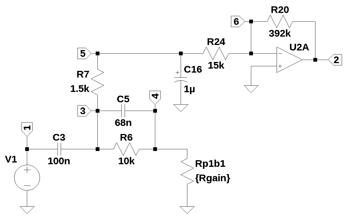
The circuit shown below is reactive branch 1. This circuit is a modified version of the circuit path analyzed in Section 37.11.1 and is a slightly modified version of the highlighted portion of circuit shown in Figure 37.15.

This circuit branch starts at the output of Op Amp \(U_{1A}\) and follows the components \(C_3\), \(R_7\) and \(R_{24}\) to the Op Amp \(U_{2A}\). Components \(R_6\), \(C_5\), \(P_1\) and \(C_{16}\) connect to circuit nodes along the branch of interest. The output of \(U_{1A}\) is replaced by the independent voltage source \(V_1\). The inverting input of \(U_{2A}\) is connected to \(R_{24}\) and this is the summing junction for other signal paths in the Klon Centaur. \(C_3\) acts as a DC block. The components, \(C_5\), \(R_6\) and \(P_1\) on node 3, and components \(R_7\) and \(C_16\) complete a low pass filter section ending at node 5.

The components,\(R_{24}\), \(R_{20}\) and \(U_{2A}\) are configured as an inverting amplifier with a gain of \(\frac{R_{20}}{R_{24}}\).

The circuit shown below is effectively a low pass filter with a DC block. \(C_3\) will block low frequencies down to DC. \(C_4\), \(R_6\) and \(R_{p1b}\) will put a zero in the transfer function along with \(C_3\). Given that there are three capacitors in the circuit, there are likely three poles in the voltage transfer function. \(C_{13}\) in the feedback of \(U_{2A}\) was omitted from the analysis so that the operation of the circuit could be analyzed without the pole created by \(R_{20}\) and \(C_{13}\) from dominating the frequency response of the transfer function.

The component \(R_{p1b1}\) in Figure 39.1 is one of the dual ganged pots in \(P_1\). The wiper of \(P_1\) is connected to ground. Node 4 in the schematic below is connected to the non-inverting input of \(U_{1B}\), but this connection is being ignored for this analysis since \(U_{1B}\) is not on the signal path we are interested in. We can still get an idea of what the components shown in the schematic are doing, but the exact location of the poles and zeros will be a little off.

Figure 39.1: Schematic of reactive branch 1.

The netlist below was exported from LTSpice.

reactive_branch_1_net_list = '''
* Klon-Centaur_sum_path1_v1.asc
V1 1 0 1
C3 3 1 100e-9
R6 4 3 10e3
C5 4 3 68e-9
R7 3 5 1.5e3
R24 6 5 15e3
C16 5 0 1e-6
Rp1b 0 4 50e3
O2a 6 0 2
R20 2 6 392e3
*C13 2 6 820e-12
'''

The MNA equations are generated from the function SymMNA.smna.

report, network_df, i_unk_df, A, X, Z = SymMNA.smna(reactive_branch_1_net_list)

The code below assembles the network equations from the MNA matrices and displays the equations.

# Put matrices into SymPy 
X = Matrix(X)
Z = Matrix(Z)

NE_sym = Eq(A*X,Z)

# display the equations
temp = ''
for i in range(shape(NE_sym.lhs)[0]):
    temp += '${:s} = {:s}$<br>'.format(latex(NE_sym.rhs[i]),latex(NE_sym.lhs[i]))
Markdown(temp)

\(0 = C_{3} s v_{1} - C_{3} s v_{3} + I_{V1}\)
\(0 = I_{O2a} + \frac{v_{2}}{R_{20}} - \frac{v_{6}}{R_{20}}\)
\(0 = - C_{3} s v_{1} + v_{3} \left(C_{3} s + C_{5} s + \frac{1}{R_{7}} + \frac{1}{R_{6}}\right) + v_{4} \left(- C_{5} s - \frac{1}{R_{6}}\right) - \frac{v_{5}}{R_{7}}\)
\(0 = v_{3} \left(- C_{5} s - \frac{1}{R_{6}}\right) + v_{4} \left(C_{5} s + \frac{1}{Rp1b} + \frac{1}{R_{6}}\right)\)
\(0 = v_{5} \left(C_{16} s + \frac{1}{R_{7}} + \frac{1}{R_{24}}\right) - \frac{v_{3}}{R_{7}} - \frac{v_{6}}{R_{24}}\)
\(0 = v_{6} \cdot \left(\frac{1}{R_{24}} + \frac{1}{R_{20}}\right) - \frac{v_{5}}{R_{24}} - \frac{v_{2}}{R_{20}}\)
\(V_{1} = v_{1}\)
\(0 = v_{6}\)

The free symbols are entered as SymPy variables and the element values are put into a dictionary.

var(str(NE_sym.free_symbols).replace('{','').replace('}',''))
element_values = SymMNA.get_part_values(network_df)

39.3.1.1 Symbolic solution

The network equations can be solved symbolically.

U_sym = solve(NE_sym,X)

Display the node voltages and dependent currents using symbolic notation.

temp = ''
for i in U_sym.keys():
    temp += '${:s} = {:s}$<br>'.format(latex(i),latex(U_sym[i]))

Markdown(temp)

\(v_{1} = V_{1}\)
\(v_{2} = \frac{- C_{3} C_{5} R_{20} R_{6} Rp1b V_{1} s^{2} - C_{3} R_{20} R_{6} V_{1} s - C_{3} R_{20} Rp1b V_{1} s}{C_{16} C_{3} C_{5} R_{24} R_{6} R_{7} Rp1b s^{3} + C_{16} C_{3} R_{24} R_{6} R_{7} s^{2} + C_{16} C_{3} R_{24} R_{7} Rp1b s^{2} + C_{16} C_{5} R_{24} R_{6} R_{7} s^{2} + C_{16} C_{5} R_{24} R_{6} Rp1b s^{2} + C_{16} R_{24} R_{6} s + C_{16} R_{24} R_{7} s + C_{16} R_{24} Rp1b s + C_{3} C_{5} R_{24} R_{6} Rp1b s^{2} + C_{3} C_{5} R_{6} R_{7} Rp1b s^{2} + C_{3} R_{24} R_{6} s + C_{3} R_{24} Rp1b s + C_{3} R_{6} R_{7} s + C_{3} R_{7} Rp1b s + C_{5} R_{24} R_{6} s + C_{5} R_{6} R_{7} s + C_{5} R_{6} Rp1b s + R_{24} + R_{6} + R_{7} + Rp1b}\)
\(v_{3} = \frac{C_{16} C_{3} C_{5} R_{24} R_{6} R_{7} Rp1b V_{1} s^{3} + C_{16} C_{3} R_{24} R_{6} R_{7} V_{1} s^{2} + C_{16} C_{3} R_{24} R_{7} Rp1b V_{1} s^{2} + C_{3} C_{5} R_{24} R_{6} Rp1b V_{1} s^{2} + C_{3} C_{5} R_{6} R_{7} Rp1b V_{1} s^{2} + C_{3} R_{24} R_{6} V_{1} s + C_{3} R_{24} Rp1b V_{1} s + C_{3} R_{6} R_{7} V_{1} s + C_{3} R_{7} Rp1b V_{1} s}{C_{16} C_{3} C_{5} R_{24} R_{6} R_{7} Rp1b s^{3} + C_{16} C_{3} R_{24} R_{6} R_{7} s^{2} + C_{16} C_{3} R_{24} R_{7} Rp1b s^{2} + C_{16} C_{5} R_{24} R_{6} R_{7} s^{2} + C_{16} C_{5} R_{24} R_{6} Rp1b s^{2} + C_{16} R_{24} R_{6} s + C_{16} R_{24} R_{7} s + C_{16} R_{24} Rp1b s + C_{3} C_{5} R_{24} R_{6} Rp1b s^{2} + C_{3} C_{5} R_{6} R_{7} Rp1b s^{2} + C_{3} R_{24} R_{6} s + C_{3} R_{24} Rp1b s + C_{3} R_{6} R_{7} s + C_{3} R_{7} Rp1b s + C_{5} R_{24} R_{6} s + C_{5} R_{6} R_{7} s + C_{5} R_{6} Rp1b s + R_{24} + R_{6} + R_{7} + Rp1b}\)
\(v_{4} = \frac{C_{16} C_{3} C_{5} R_{24} R_{6} R_{7} Rp1b V_{1} s^{3} + C_{16} C_{3} R_{24} R_{7} Rp1b V_{1} s^{2} + C_{3} C_{5} R_{24} R_{6} Rp1b V_{1} s^{2} + C_{3} C_{5} R_{6} R_{7} Rp1b V_{1} s^{2} + C_{3} R_{24} Rp1b V_{1} s + C_{3} R_{7} Rp1b V_{1} s}{C_{16} C_{3} C_{5} R_{24} R_{6} R_{7} Rp1b s^{3} + C_{16} C_{3} R_{24} R_{6} R_{7} s^{2} + C_{16} C_{3} R_{24} R_{7} Rp1b s^{2} + C_{16} C_{5} R_{24} R_{6} R_{7} s^{2} + C_{16} C_{5} R_{24} R_{6} Rp1b s^{2} + C_{16} R_{24} R_{6} s + C_{16} R_{24} R_{7} s + C_{16} R_{24} Rp1b s + C_{3} C_{5} R_{24} R_{6} Rp1b s^{2} + C_{3} C_{5} R_{6} R_{7} Rp1b s^{2} + C_{3} R_{24} R_{6} s + C_{3} R_{24} Rp1b s + C_{3} R_{6} R_{7} s + C_{3} R_{7} Rp1b s + C_{5} R_{24} R_{6} s + C_{5} R_{6} R_{7} s + C_{5} R_{6} Rp1b s + R_{24} + R_{6} + R_{7} + Rp1b}\)
\(v_{5} = \frac{C_{3} C_{5} R_{24} R_{6} Rp1b V_{1} s^{2} + C_{3} R_{24} R_{6} V_{1} s + C_{3} R_{24} Rp1b V_{1} s}{C_{16} C_{3} C_{5} R_{24} R_{6} R_{7} Rp1b s^{3} + C_{16} C_{3} R_{24} R_{6} R_{7} s^{2} + C_{16} C_{3} R_{24} R_{7} Rp1b s^{2} + C_{16} C_{5} R_{24} R_{6} R_{7} s^{2} + C_{16} C_{5} R_{24} R_{6} Rp1b s^{2} + C_{16} R_{24} R_{6} s + C_{16} R_{24} R_{7} s + C_{16} R_{24} Rp1b s + C_{3} C_{5} R_{24} R_{6} Rp1b s^{2} + C_{3} C_{5} R_{6} R_{7} Rp1b s^{2} + C_{3} R_{24} R_{6} s + C_{3} R_{24} Rp1b s + C_{3} R_{6} R_{7} s + C_{3} R_{7} Rp1b s + C_{5} R_{24} R_{6} s + C_{5} R_{6} R_{7} s + C_{5} R_{6} Rp1b s + R_{24} + R_{6} + R_{7} + Rp1b}\)
\(v_{6} = 0\)
\(I_{V1} = \frac{- C_{16} C_{3} C_{5} R_{24} R_{6} R_{7} V_{1} s^{3} - C_{16} C_{3} C_{5} R_{24} R_{6} Rp1b V_{1} s^{3} - C_{16} C_{3} R_{24} R_{6} V_{1} s^{2} - C_{16} C_{3} R_{24} R_{7} V_{1} s^{2} - C_{16} C_{3} R_{24} Rp1b V_{1} s^{2} - C_{3} C_{5} R_{24} R_{6} V_{1} s^{2} - C_{3} C_{5} R_{6} R_{7} V_{1} s^{2} - C_{3} C_{5} R_{6} Rp1b V_{1} s^{2} - C_{3} R_{24} V_{1} s - C_{3} R_{6} V_{1} s - C_{3} R_{7} V_{1} s - C_{3} Rp1b V_{1} s}{C_{16} C_{3} C_{5} R_{24} R_{6} R_{7} Rp1b s^{3} + C_{16} C_{3} R_{24} R_{6} R_{7} s^{2} + C_{16} C_{3} R_{24} R_{7} Rp1b s^{2} + C_{16} C_{5} R_{24} R_{6} R_{7} s^{2} + C_{16} C_{5} R_{24} R_{6} Rp1b s^{2} + C_{16} R_{24} R_{6} s + C_{16} R_{24} R_{7} s + C_{16} R_{24} Rp1b s + C_{3} C_{5} R_{24} R_{6} Rp1b s^{2} + C_{3} C_{5} R_{6} R_{7} Rp1b s^{2} + C_{3} R_{24} R_{6} s + C_{3} R_{24} Rp1b s + C_{3} R_{6} R_{7} s + C_{3} R_{7} Rp1b s + C_{5} R_{24} R_{6} s + C_{5} R_{6} R_{7} s + C_{5} R_{6} Rp1b s + R_{24} + R_{6} + R_{7} + Rp1b}\)
\(I_{O2a} = \frac{C_{3} C_{5} R_{6} Rp1b V_{1} s^{2} + C_{3} R_{6} V_{1} s + C_{3} Rp1b V_{1} s}{C_{16} C_{3} C_{5} R_{24} R_{6} R_{7} Rp1b s^{3} + C_{16} C_{3} R_{24} R_{6} R_{7} s^{2} + C_{16} C_{3} R_{24} R_{7} Rp1b s^{2} + C_{16} C_{5} R_{24} R_{6} R_{7} s^{2} + C_{16} C_{5} R_{24} R_{6} Rp1b s^{2} + C_{16} R_{24} R_{6} s + C_{16} R_{24} R_{7} s + C_{16} R_{24} Rp1b s + C_{3} C_{5} R_{24} R_{6} Rp1b s^{2} + C_{3} C_{5} R_{6} R_{7} Rp1b s^{2} + C_{3} R_{24} R_{6} s + C_{3} R_{24} Rp1b s + C_{3} R_{6} R_{7} s + C_{3} R_{7} Rp1b s + C_{5} R_{24} R_{6} s + C_{5} R_{6} R_{7} s + C_{5} R_{6} Rp1b s + R_{24} + R_{6} + R_{7} + Rp1b}\)

The network transfer function, \(H(s)=\frac {v_2(s)}{v_1(s)}\) is:

H_sym = (U_sym[v2]/U_sym[v1]).cancel()
Markdown('$H(s)={:s}$'.format(latex(H_sym)))

\(H(s)=\frac{- C_{3} C_{5} R_{20} R_{6} Rp1b s^{2} - C_{3} R_{20} R_{6} s - C_{3} R_{20} Rp1b s}{C_{16} C_{3} C_{5} R_{24} R_{6} R_{7} Rp1b s^{3} + C_{16} C_{3} R_{24} R_{6} R_{7} s^{2} + C_{16} C_{3} R_{24} R_{7} Rp1b s^{2} + C_{16} C_{5} R_{24} R_{6} R_{7} s^{2} + C_{16} C_{5} R_{24} R_{6} Rp1b s^{2} + C_{16} R_{24} R_{6} s + C_{16} R_{24} R_{7} s + C_{16} R_{24} Rp1b s + C_{3} C_{5} R_{24} R_{6} Rp1b s^{2} + C_{3} C_{5} R_{6} R_{7} Rp1b s^{2} + C_{3} R_{24} R_{6} s + C_{3} R_{24} Rp1b s + C_{3} R_{6} R_{7} s + C_{3} R_{7} Rp1b s + C_{5} R_{24} R_{6} s + C_{5} R_{6} R_{7} s + C_{5} R_{6} Rp1b s + R_{24} + R_{6} + R_{7} + Rp1b}\)

The numerator is a second order polynomial and the denominator is a third order polynomial. Generally, the order of the dominator is equal to the number of reactive elements in the circuit; sometimes roots of the numerator will exactly cancel with a root of the denominator polynomial. The roots of the numerator polynomial are called the zeros of the transfer function and the roots of the denominator are called the poles of the transfer function.

H_sym_num, H_sym_denom = fraction(H_sym,s) #returns numerator and denominator

39.3.1.2 Numerator Polynomial of \(H_{sym}(s)\)

The numerator polynomial is:

Markdown('$N(s)={:s}$'.format(latex(H_sym_num)))

\(N(s)=- C_{3} C_{5} R_{20} R_{6} Rp1b s^{2} - C_{3} R_{20} R_{6} s - C_{3} R_{20} Rp1b s\)

The coefficients of each Laplace term can be equated to the variables \(b_2\), \(b_1\) and \(b_0\) in the expression:

\(b_2s^{2}+b_1s+b_0\)

where \(b_2\), \(b_1\) and \(b_0\) are:

b2 = H_sym_num.coeff(s**2)
b1 = H_sym_num.coeff(s**1)
b0 = (H_sym_num - b1*s*1 - b2*s**2).expand()

Markdown('<p>$b_2={:s}$</p><p>$b_1={:s}$</p><p>$b_0={:s}$</p>'.format(latex(b2),latex(b1),latex(b0)))

\(b_2=- C_{3} C_{5} R_{20} R_{6} Rp1b\)

\(b_1=- C_{3} R_{20} R_{6} - C_{3} R_{20} Rp1b\)

\(b_0=0\)

The roots of the numerator polynomial can easily be found with SymPy. This filter has two transmission zeros, which can be found using the solve function on the numerator polynomial.

num_root_sym = solve(H_sym_num,s)

Markdown('There are {:d} zeros, which are:\
    <p>$z_0={:s}$</p><p>$z_1={:s}$</p>'.format(len(num_root_sym),latex(num_root_sym[0]),latex(num_root_sym[1])))

There are 2 zeros, which are:

\(z_0=0\)

\(z_1=\frac{- R_{6} - Rp1b}{C_{5} R_{6} Rp1b}\)

\(C_3\) is responsible for the zero at \(\omega=0\) since this capacitor provids an open circuit at DC.

39.3.1.3 Denominator Polynomial of \(H_{sym}(s)\)

The denominator polynomial of the transfer function is called the characteristic polynomial. The roots of the denominator, also called poles of the system, determine the system’s stability. If any of these roots have a positive real part, the system is unstable, meaning its output will grow unbounded. The roots also influence how the system responds to changes in input (the transient response). They affect things like how quickly the system settles to a new state, whether it oscillates, and the damping of those oscillations. Each root of the characteristic polynomial corresponds to a natural mode of the system.

The denominator polynomial is:

Markdown('$D(s)={:s}$'.format(latex(H_sym_denom)))

\(D(s)=C_{16} C_{3} C_{5} R_{24} R_{6} R_{7} Rp1b s^{3} + C_{16} C_{3} R_{24} R_{6} R_{7} s^{2} + C_{16} C_{3} R_{24} R_{7} Rp1b s^{2} + C_{16} C_{5} R_{24} R_{6} R_{7} s^{2} + C_{16} C_{5} R_{24} R_{6} Rp1b s^{2} + C_{16} R_{24} R_{6} s + C_{16} R_{24} R_{7} s + C_{16} R_{24} Rp1b s + C_{3} C_{5} R_{24} R_{6} Rp1b s^{2} + C_{3} C_{5} R_{6} R_{7} Rp1b s^{2} + C_{3} R_{24} R_{6} s + C_{3} R_{24} Rp1b s + C_{3} R_{6} R_{7} s + C_{3} R_{7} Rp1b s + C_{5} R_{24} R_{6} s + C_{5} R_{6} R_{7} s + C_{5} R_{6} Rp1b s + R_{24} + R_{6} + R_{7} + Rp1b\)

The coefficients of each Laplace term can be equated to the variables \(a_3\), \(a_2\), \(a_1\) and \(a_0\) in the expression:

\(a_3s^3+a_2s^2+a_1s+a_0\)

where \(a_3\), \(a_2\), \(a_1\) and \(a_0\) are:

a3 = H_sym_denom.coeff(s**3)
a2 = H_sym_denom.coeff(s**2)
a1 = H_sym_denom.coeff(s**1)
a0 = (H_sym_denom - a1*s*1 - a2*s**2 - a3*s**3).expand()
Markdown('<p>$a_3={:s}$</p><p>$a_2={:s}$</p><p>\
    $a_1={:s}$</p><p>$a_0={:s}$</p>'.format(latex(a3),
    latex(a2),latex(a1),latex(a0)))

\(a_3=C_{16} C_{3} C_{5} R_{24} R_{6} R_{7} Rp1b\)

\(a_2=C_{16} C_{3} R_{24} R_{6} R_{7} + C_{16} C_{3} R_{24} R_{7} Rp1b + C_{16} C_{5} R_{24} R_{6} R_{7} + C_{16} C_{5} R_{24} R_{6} Rp1b + C_{3} C_{5} R_{24} R_{6} Rp1b + C_{3} C_{5} R_{6} R_{7} Rp1b\)

\(a_1=C_{16} R_{24} R_{6} + C_{16} R_{24} R_{7} + C_{16} R_{24} Rp1b + C_{3} R_{24} R_{6} + C_{3} R_{24} Rp1b + C_{3} R_{6} R_{7} + C_{3} R_{7} Rp1b + C_{5} R_{24} R_{6} + C_{5} R_{6} R_{7} + C_{5} R_{6} Rp1b\)

\(a_0=R_{24} + R_{6} + R_{7} + Rp1b\)

The roots of the denominator polynomial, which are the poles of the transfer function, can be found with SymPy.

denom_root_sym = solve(H_sym_denom,s)

Markdown('There are {:d} poles, which are:\
    <p>$p_0={:s}$</p><p>$p_1={:s}$</p><p>$p_2={:s}$</p>'.format(len(denom_root_sym),latex(denom_root_sym[0]),latex(denom_root_sym[1]),latex(denom_root_sym[2])))

There are 3 poles, which are:

\(p_0=- \frac{- \frac{3 \left(C_{16} R_{24} R_{6} + C_{16} R_{24} R_{7} + C_{16} R_{24} Rp1b + C_{3} R_{24} R_{6} + C_{3} R_{24} Rp1b + C_{3} R_{6} R_{7} + C_{3} R_{7} Rp1b + C_{5} R_{24} R_{6} + C_{5} R_{6} R_{7} + C_{5} R_{6} Rp1b\right)}{C_{16} C_{3} C_{5} R_{24} R_{6} R_{7} Rp1b} + \frac{\left(C_{16} C_{3} R_{24} R_{6} R_{7} + C_{16} C_{3} R_{24} R_{7} Rp1b + C_{16} C_{5} R_{24} R_{6} R_{7} + C_{16} C_{5} R_{24} R_{6} Rp1b + C_{3} C_{5} R_{24} R_{6} Rp1b + C_{3} C_{5} R_{6} R_{7} Rp1b\right)^{2}}{C_{16}^{2} C_{3}^{2} C_{5}^{2} R_{24}^{2} R_{6}^{2} R_{7}^{2} Rp1b^{2}}}{3 \sqrt[3]{\frac{\sqrt{- 4 \left(- \frac{3 \left(C_{16} R_{24} R_{6} + C_{16} R_{24} R_{7} + C_{16} R_{24} Rp1b + C_{3} R_{24} R_{6} + C_{3} R_{24} Rp1b + C_{3} R_{6} R_{7} + C_{3} R_{7} Rp1b + C_{5} R_{24} R_{6} + C_{5} R_{6} R_{7} + C_{5} R_{6} Rp1b\right)}{C_{16} C_{3} C_{5} R_{24} R_{6} R_{7} Rp1b} + \frac{\left(C_{16} C_{3} R_{24} R_{6} R_{7} + C_{16} C_{3} R_{24} R_{7} Rp1b + C_{16} C_{5} R_{24} R_{6} R_{7} + C_{16} C_{5} R_{24} R_{6} Rp1b + C_{3} C_{5} R_{24} R_{6} Rp1b + C_{3} C_{5} R_{6} R_{7} Rp1b\right)^{2}}{C_{16}^{2} C_{3}^{2} C_{5}^{2} R_{24}^{2} R_{6}^{2} R_{7}^{2} Rp1b^{2}}\right)^{3} + \left(\frac{27 \left(R_{24} + R_{6} + R_{7} + Rp1b\right)}{C_{16} C_{3} C_{5} R_{24} R_{6} R_{7} Rp1b} - \frac{9 \left(C_{16} C_{3} R_{24} R_{6} R_{7} + C_{16} C_{3} R_{24} R_{7} Rp1b + C_{16} C_{5} R_{24} R_{6} R_{7} + C_{16} C_{5} R_{24} R_{6} Rp1b + C_{3} C_{5} R_{24} R_{6} Rp1b + C_{3} C_{5} R_{6} R_{7} Rp1b\right) \left(C_{16} R_{24} R_{6} + C_{16} R_{24} R_{7} + C_{16} R_{24} Rp1b + C_{3} R_{24} R_{6} + C_{3} R_{24} Rp1b + C_{3} R_{6} R_{7} + C_{3} R_{7} Rp1b + C_{5} R_{24} R_{6} + C_{5} R_{6} R_{7} + C_{5} R_{6} Rp1b\right)}{C_{16}^{2} C_{3}^{2} C_{5}^{2} R_{24}^{2} R_{6}^{2} R_{7}^{2} Rp1b^{2}} + \frac{2 \left(C_{16} C_{3} R_{24} R_{6} R_{7} + C_{16} C_{3} R_{24} R_{7} Rp1b + C_{16} C_{5} R_{24} R_{6} R_{7} + C_{16} C_{5} R_{24} R_{6} Rp1b + C_{3} C_{5} R_{24} R_{6} Rp1b + C_{3} C_{5} R_{6} R_{7} Rp1b\right)^{3}}{C_{16}^{3} C_{3}^{3} C_{5}^{3} R_{24}^{3} R_{6}^{3} R_{7}^{3} Rp1b^{3}}\right)^{2}}}{2} + \frac{27 \left(R_{24} + R_{6} + R_{7} + Rp1b\right)}{2 C_{16} C_{3} C_{5} R_{24} R_{6} R_{7} Rp1b} - \frac{9 \left(C_{16} C_{3} R_{24} R_{6} R_{7} + C_{16} C_{3} R_{24} R_{7} Rp1b + C_{16} C_{5} R_{24} R_{6} R_{7} + C_{16} C_{5} R_{24} R_{6} Rp1b + C_{3} C_{5} R_{24} R_{6} Rp1b + C_{3} C_{5} R_{6} R_{7} Rp1b\right) \left(C_{16} R_{24} R_{6} + C_{16} R_{24} R_{7} + C_{16} R_{24} Rp1b + C_{3} R_{24} R_{6} + C_{3} R_{24} Rp1b + C_{3} R_{6} R_{7} + C_{3} R_{7} Rp1b + C_{5} R_{24} R_{6} + C_{5} R_{6} R_{7} + C_{5} R_{6} Rp1b\right)}{2 C_{16}^{2} C_{3}^{2} C_{5}^{2} R_{24}^{2} R_{6}^{2} R_{7}^{2} Rp1b^{2}} + \frac{\left(C_{16} C_{3} R_{24} R_{6} R_{7} + C_{16} C_{3} R_{24} R_{7} Rp1b + C_{16} C_{5} R_{24} R_{6} R_{7} + C_{16} C_{5} R_{24} R_{6} Rp1b + C_{3} C_{5} R_{24} R_{6} Rp1b + C_{3} C_{5} R_{6} R_{7} Rp1b\right)^{3}}{C_{16}^{3} C_{3}^{3} C_{5}^{3} R_{24}^{3} R_{6}^{3} R_{7}^{3} Rp1b^{3}}}} - \frac{\sqrt[3]{\frac{\sqrt{- 4 \left(- \frac{3 \left(C_{16} R_{24} R_{6} + C_{16} R_{24} R_{7} + C_{16} R_{24} Rp1b + C_{3} R_{24} R_{6} + C_{3} R_{24} Rp1b + C_{3} R_{6} R_{7} + C_{3} R_{7} Rp1b + C_{5} R_{24} R_{6} + C_{5} R_{6} R_{7} + C_{5} R_{6} Rp1b\right)}{C_{16} C_{3} C_{5} R_{24} R_{6} R_{7} Rp1b} + \frac{\left(C_{16} C_{3} R_{24} R_{6} R_{7} + C_{16} C_{3} R_{24} R_{7} Rp1b + C_{16} C_{5} R_{24} R_{6} R_{7} + C_{16} C_{5} R_{24} R_{6} Rp1b + C_{3} C_{5} R_{24} R_{6} Rp1b + C_{3} C_{5} R_{6} R_{7} Rp1b\right)^{2}}{C_{16}^{2} C_{3}^{2} C_{5}^{2} R_{24}^{2} R_{6}^{2} R_{7}^{2} Rp1b^{2}}\right)^{3} + \left(\frac{27 \left(R_{24} + R_{6} + R_{7} + Rp1b\right)}{C_{16} C_{3} C_{5} R_{24} R_{6} R_{7} Rp1b} - \frac{9 \left(C_{16} C_{3} R_{24} R_{6} R_{7} + C_{16} C_{3} R_{24} R_{7} Rp1b + C_{16} C_{5} R_{24} R_{6} R_{7} + C_{16} C_{5} R_{24} R_{6} Rp1b + C_{3} C_{5} R_{24} R_{6} Rp1b + C_{3} C_{5} R_{6} R_{7} Rp1b\right) \left(C_{16} R_{24} R_{6} + C_{16} R_{24} R_{7} + C_{16} R_{24} Rp1b + C_{3} R_{24} R_{6} + C_{3} R_{24} Rp1b + C_{3} R_{6} R_{7} + C_{3} R_{7} Rp1b + C_{5} R_{24} R_{6} + C_{5} R_{6} R_{7} + C_{5} R_{6} Rp1b\right)}{C_{16}^{2} C_{3}^{2} C_{5}^{2} R_{24}^{2} R_{6}^{2} R_{7}^{2} Rp1b^{2}} + \frac{2 \left(C_{16} C_{3} R_{24} R_{6} R_{7} + C_{16} C_{3} R_{24} R_{7} Rp1b + C_{16} C_{5} R_{24} R_{6} R_{7} + C_{16} C_{5} R_{24} R_{6} Rp1b + C_{3} C_{5} R_{24} R_{6} Rp1b + C_{3} C_{5} R_{6} R_{7} Rp1b\right)^{3}}{C_{16}^{3} C_{3}^{3} C_{5}^{3} R_{24}^{3} R_{6}^{3} R_{7}^{3} Rp1b^{3}}\right)^{2}}}{2} + \frac{27 \left(R_{24} + R_{6} + R_{7} + Rp1b\right)}{2 C_{16} C_{3} C_{5} R_{24} R_{6} R_{7} Rp1b} - \frac{9 \left(C_{16} C_{3} R_{24} R_{6} R_{7} + C_{16} C_{3} R_{24} R_{7} Rp1b + C_{16} C_{5} R_{24} R_{6} R_{7} + C_{16} C_{5} R_{24} R_{6} Rp1b + C_{3} C_{5} R_{24} R_{6} Rp1b + C_{3} C_{5} R_{6} R_{7} Rp1b\right) \left(C_{16} R_{24} R_{6} + C_{16} R_{24} R_{7} + C_{16} R_{24} Rp1b + C_{3} R_{24} R_{6} + C_{3} R_{24} Rp1b + C_{3} R_{6} R_{7} + C_{3} R_{7} Rp1b + C_{5} R_{24} R_{6} + C_{5} R_{6} R_{7} + C_{5} R_{6} Rp1b\right)}{2 C_{16}^{2} C_{3}^{2} C_{5}^{2} R_{24}^{2} R_{6}^{2} R_{7}^{2} Rp1b^{2}} + \frac{\left(C_{16} C_{3} R_{24} R_{6} R_{7} + C_{16} C_{3} R_{24} R_{7} Rp1b + C_{16} C_{5} R_{24} R_{6} R_{7} + C_{16} C_{5} R_{24} R_{6} Rp1b + C_{3} C_{5} R_{24} R_{6} Rp1b + C_{3} C_{5} R_{6} R_{7} Rp1b\right)^{3}}{C_{16}^{3} C_{3}^{3} C_{5}^{3} R_{24}^{3} R_{6}^{3} R_{7}^{3} Rp1b^{3}}}}{3} - \frac{C_{16} C_{3} R_{24} R_{6} R_{7} + C_{16} C_{3} R_{24} R_{7} Rp1b + C_{16} C_{5} R_{24} R_{6} R_{7} + C_{16} C_{5} R_{24} R_{6} Rp1b + C_{3} C_{5} R_{24} R_{6} Rp1b + C_{3} C_{5} R_{6} R_{7} Rp1b}{3 C_{16} C_{3} C_{5} R_{24} R_{6} R_{7} Rp1b}\)

\(p_1=- \frac{- \frac{3 \left(C_{16} R_{24} R_{6} + C_{16} R_{24} R_{7} + C_{16} R_{24} Rp1b + C_{3} R_{24} R_{6} + C_{3} R_{24} Rp1b + C_{3} R_{6} R_{7} + C_{3} R_{7} Rp1b + C_{5} R_{24} R_{6} + C_{5} R_{6} R_{7} + C_{5} R_{6} Rp1b\right)}{C_{16} C_{3} C_{5} R_{24} R_{6} R_{7} Rp1b} + \frac{\left(C_{16} C_{3} R_{24} R_{6} R_{7} + C_{16} C_{3} R_{24} R_{7} Rp1b + C_{16} C_{5} R_{24} R_{6} R_{7} + C_{16} C_{5} R_{24} R_{6} Rp1b + C_{3} C_{5} R_{24} R_{6} Rp1b + C_{3} C_{5} R_{6} R_{7} Rp1b\right)^{2}}{C_{16}^{2} C_{3}^{2} C_{5}^{2} R_{24}^{2} R_{6}^{2} R_{7}^{2} Rp1b^{2}}}{3 \left(- \frac{1}{2} - \frac{\sqrt{3} i}{2}\right) \sqrt[3]{\frac{\sqrt{- 4 \left(- \frac{3 \left(C_{16} R_{24} R_{6} + C_{16} R_{24} R_{7} + C_{16} R_{24} Rp1b + C_{3} R_{24} R_{6} + C_{3} R_{24} Rp1b + C_{3} R_{6} R_{7} + C_{3} R_{7} Rp1b + C_{5} R_{24} R_{6} + C_{5} R_{6} R_{7} + C_{5} R_{6} Rp1b\right)}{C_{16} C_{3} C_{5} R_{24} R_{6} R_{7} Rp1b} + \frac{\left(C_{16} C_{3} R_{24} R_{6} R_{7} + C_{16} C_{3} R_{24} R_{7} Rp1b + C_{16} C_{5} R_{24} R_{6} R_{7} + C_{16} C_{5} R_{24} R_{6} Rp1b + C_{3} C_{5} R_{24} R_{6} Rp1b + C_{3} C_{5} R_{6} R_{7} Rp1b\right)^{2}}{C_{16}^{2} C_{3}^{2} C_{5}^{2} R_{24}^{2} R_{6}^{2} R_{7}^{2} Rp1b^{2}}\right)^{3} + \left(\frac{27 \left(R_{24} + R_{6} + R_{7} + Rp1b\right)}{C_{16} C_{3} C_{5} R_{24} R_{6} R_{7} Rp1b} - \frac{9 \left(C_{16} C_{3} R_{24} R_{6} R_{7} + C_{16} C_{3} R_{24} R_{7} Rp1b + C_{16} C_{5} R_{24} R_{6} R_{7} + C_{16} C_{5} R_{24} R_{6} Rp1b + C_{3} C_{5} R_{24} R_{6} Rp1b + C_{3} C_{5} R_{6} R_{7} Rp1b\right) \left(C_{16} R_{24} R_{6} + C_{16} R_{24} R_{7} + C_{16} R_{24} Rp1b + C_{3} R_{24} R_{6} + C_{3} R_{24} Rp1b + C_{3} R_{6} R_{7} + C_{3} R_{7} Rp1b + C_{5} R_{24} R_{6} + C_{5} R_{6} R_{7} + C_{5} R_{6} Rp1b\right)}{C_{16}^{2} C_{3}^{2} C_{5}^{2} R_{24}^{2} R_{6}^{2} R_{7}^{2} Rp1b^{2}} + \frac{2 \left(C_{16} C_{3} R_{24} R_{6} R_{7} + C_{16} C_{3} R_{24} R_{7} Rp1b + C_{16} C_{5} R_{24} R_{6} R_{7} + C_{16} C_{5} R_{24} R_{6} Rp1b + C_{3} C_{5} R_{24} R_{6} Rp1b + C_{3} C_{5} R_{6} R_{7} Rp1b\right)^{3}}{C_{16}^{3} C_{3}^{3} C_{5}^{3} R_{24}^{3} R_{6}^{3} R_{7}^{3} Rp1b^{3}}\right)^{2}}}{2} + \frac{27 \left(R_{24} + R_{6} + R_{7} + Rp1b\right)}{2 C_{16} C_{3} C_{5} R_{24} R_{6} R_{7} Rp1b} - \frac{9 \left(C_{16} C_{3} R_{24} R_{6} R_{7} + C_{16} C_{3} R_{24} R_{7} Rp1b + C_{16} C_{5} R_{24} R_{6} R_{7} + C_{16} C_{5} R_{24} R_{6} Rp1b + C_{3} C_{5} R_{24} R_{6} Rp1b + C_{3} C_{5} R_{6} R_{7} Rp1b\right) \left(C_{16} R_{24} R_{6} + C_{16} R_{24} R_{7} + C_{16} R_{24} Rp1b + C_{3} R_{24} R_{6} + C_{3} R_{24} Rp1b + C_{3} R_{6} R_{7} + C_{3} R_{7} Rp1b + C_{5} R_{24} R_{6} + C_{5} R_{6} R_{7} + C_{5} R_{6} Rp1b\right)}{2 C_{16}^{2} C_{3}^{2} C_{5}^{2} R_{24}^{2} R_{6}^{2} R_{7}^{2} Rp1b^{2}} + \frac{\left(C_{16} C_{3} R_{24} R_{6} R_{7} + C_{16} C_{3} R_{24} R_{7} Rp1b + C_{16} C_{5} R_{24} R_{6} R_{7} + C_{16} C_{5} R_{24} R_{6} Rp1b + C_{3} C_{5} R_{24} R_{6} Rp1b + C_{3} C_{5} R_{6} R_{7} Rp1b\right)^{3}}{C_{16}^{3} C_{3}^{3} C_{5}^{3} R_{24}^{3} R_{6}^{3} R_{7}^{3} Rp1b^{3}}}} - \frac{\left(- \frac{1}{2} - \frac{\sqrt{3} i}{2}\right) \sqrt[3]{\frac{\sqrt{- 4 \left(- \frac{3 \left(C_{16} R_{24} R_{6} + C_{16} R_{24} R_{7} + C_{16} R_{24} Rp1b + C_{3} R_{24} R_{6} + C_{3} R_{24} Rp1b + C_{3} R_{6} R_{7} + C_{3} R_{7} Rp1b + C_{5} R_{24} R_{6} + C_{5} R_{6} R_{7} + C_{5} R_{6} Rp1b\right)}{C_{16} C_{3} C_{5} R_{24} R_{6} R_{7} Rp1b} + \frac{\left(C_{16} C_{3} R_{24} R_{6} R_{7} + C_{16} C_{3} R_{24} R_{7} Rp1b + C_{16} C_{5} R_{24} R_{6} R_{7} + C_{16} C_{5} R_{24} R_{6} Rp1b + C_{3} C_{5} R_{24} R_{6} Rp1b + C_{3} C_{5} R_{6} R_{7} Rp1b\right)^{2}}{C_{16}^{2} C_{3}^{2} C_{5}^{2} R_{24}^{2} R_{6}^{2} R_{7}^{2} Rp1b^{2}}\right)^{3} + \left(\frac{27 \left(R_{24} + R_{6} + R_{7} + Rp1b\right)}{C_{16} C_{3} C_{5} R_{24} R_{6} R_{7} Rp1b} - \frac{9 \left(C_{16} C_{3} R_{24} R_{6} R_{7} + C_{16} C_{3} R_{24} R_{7} Rp1b + C_{16} C_{5} R_{24} R_{6} R_{7} + C_{16} C_{5} R_{24} R_{6} Rp1b + C_{3} C_{5} R_{24} R_{6} Rp1b + C_{3} C_{5} R_{6} R_{7} Rp1b\right) \left(C_{16} R_{24} R_{6} + C_{16} R_{24} R_{7} + C_{16} R_{24} Rp1b + C_{3} R_{24} R_{6} + C_{3} R_{24} Rp1b + C_{3} R_{6} R_{7} + C_{3} R_{7} Rp1b + C_{5} R_{24} R_{6} + C_{5} R_{6} R_{7} + C_{5} R_{6} Rp1b\right)}{C_{16}^{2} C_{3}^{2} C_{5}^{2} R_{24}^{2} R_{6}^{2} R_{7}^{2} Rp1b^{2}} + \frac{2 \left(C_{16} C_{3} R_{24} R_{6} R_{7} + C_{16} C_{3} R_{24} R_{7} Rp1b + C_{16} C_{5} R_{24} R_{6} R_{7} + C_{16} C_{5} R_{24} R_{6} Rp1b + C_{3} C_{5} R_{24} R_{6} Rp1b + C_{3} C_{5} R_{6} R_{7} Rp1b\right)^{3}}{C_{16}^{3} C_{3}^{3} C_{5}^{3} R_{24}^{3} R_{6}^{3} R_{7}^{3} Rp1b^{3}}\right)^{2}}}{2} + \frac{27 \left(R_{24} + R_{6} + R_{7} + Rp1b\right)}{2 C_{16} C_{3} C_{5} R_{24} R_{6} R_{7} Rp1b} - \frac{9 \left(C_{16} C_{3} R_{24} R_{6} R_{7} + C_{16} C_{3} R_{24} R_{7} Rp1b + C_{16} C_{5} R_{24} R_{6} R_{7} + C_{16} C_{5} R_{24} R_{6} Rp1b + C_{3} C_{5} R_{24} R_{6} Rp1b + C_{3} C_{5} R_{6} R_{7} Rp1b\right) \left(C_{16} R_{24} R_{6} + C_{16} R_{24} R_{7} + C_{16} R_{24} Rp1b + C_{3} R_{24} R_{6} + C_{3} R_{24} Rp1b + C_{3} R_{6} R_{7} + C_{3} R_{7} Rp1b + C_{5} R_{24} R_{6} + C_{5} R_{6} R_{7} + C_{5} R_{6} Rp1b\right)}{2 C_{16}^{2} C_{3}^{2} C_{5}^{2} R_{24}^{2} R_{6}^{2} R_{7}^{2} Rp1b^{2}} + \frac{\left(C_{16} C_{3} R_{24} R_{6} R_{7} + C_{16} C_{3} R_{24} R_{7} Rp1b + C_{16} C_{5} R_{24} R_{6} R_{7} + C_{16} C_{5} R_{24} R_{6} Rp1b + C_{3} C_{5} R_{24} R_{6} Rp1b + C_{3} C_{5} R_{6} R_{7} Rp1b\right)^{3}}{C_{16}^{3} C_{3}^{3} C_{5}^{3} R_{24}^{3} R_{6}^{3} R_{7}^{3} Rp1b^{3}}}}{3} - \frac{C_{16} C_{3} R_{24} R_{6} R_{7} + C_{16} C_{3} R_{24} R_{7} Rp1b + C_{16} C_{5} R_{24} R_{6} R_{7} + C_{16} C_{5} R_{24} R_{6} Rp1b + C_{3} C_{5} R_{24} R_{6} Rp1b + C_{3} C_{5} R_{6} R_{7} Rp1b}{3 C_{16} C_{3} C_{5} R_{24} R_{6} R_{7} Rp1b}\)

\(p_2=- \frac{- \frac{3 \left(C_{16} R_{24} R_{6} + C_{16} R_{24} R_{7} + C_{16} R_{24} Rp1b + C_{3} R_{24} R_{6} + C_{3} R_{24} Rp1b + C_{3} R_{6} R_{7} + C_{3} R_{7} Rp1b + C_{5} R_{24} R_{6} + C_{5} R_{6} R_{7} + C_{5} R_{6} Rp1b\right)}{C_{16} C_{3} C_{5} R_{24} R_{6} R_{7} Rp1b} + \frac{\left(C_{16} C_{3} R_{24} R_{6} R_{7} + C_{16} C_{3} R_{24} R_{7} Rp1b + C_{16} C_{5} R_{24} R_{6} R_{7} + C_{16} C_{5} R_{24} R_{6} Rp1b + C_{3} C_{5} R_{24} R_{6} Rp1b + C_{3} C_{5} R_{6} R_{7} Rp1b\right)^{2}}{C_{16}^{2} C_{3}^{2} C_{5}^{2} R_{24}^{2} R_{6}^{2} R_{7}^{2} Rp1b^{2}}}{3 \left(- \frac{1}{2} + \frac{\sqrt{3} i}{2}\right) \sqrt[3]{\frac{\sqrt{- 4 \left(- \frac{3 \left(C_{16} R_{24} R_{6} + C_{16} R_{24} R_{7} + C_{16} R_{24} Rp1b + C_{3} R_{24} R_{6} + C_{3} R_{24} Rp1b + C_{3} R_{6} R_{7} + C_{3} R_{7} Rp1b + C_{5} R_{24} R_{6} + C_{5} R_{6} R_{7} + C_{5} R_{6} Rp1b\right)}{C_{16} C_{3} C_{5} R_{24} R_{6} R_{7} Rp1b} + \frac{\left(C_{16} C_{3} R_{24} R_{6} R_{7} + C_{16} C_{3} R_{24} R_{7} Rp1b + C_{16} C_{5} R_{24} R_{6} R_{7} + C_{16} C_{5} R_{24} R_{6} Rp1b + C_{3} C_{5} R_{24} R_{6} Rp1b + C_{3} C_{5} R_{6} R_{7} Rp1b\right)^{2}}{C_{16}^{2} C_{3}^{2} C_{5}^{2} R_{24}^{2} R_{6}^{2} R_{7}^{2} Rp1b^{2}}\right)^{3} + \left(\frac{27 \left(R_{24} + R_{6} + R_{7} + Rp1b\right)}{C_{16} C_{3} C_{5} R_{24} R_{6} R_{7} Rp1b} - \frac{9 \left(C_{16} C_{3} R_{24} R_{6} R_{7} + C_{16} C_{3} R_{24} R_{7} Rp1b + C_{16} C_{5} R_{24} R_{6} R_{7} + C_{16} C_{5} R_{24} R_{6} Rp1b + C_{3} C_{5} R_{24} R_{6} Rp1b + C_{3} C_{5} R_{6} R_{7} Rp1b\right) \left(C_{16} R_{24} R_{6} + C_{16} R_{24} R_{7} + C_{16} R_{24} Rp1b + C_{3} R_{24} R_{6} + C_{3} R_{24} Rp1b + C_{3} R_{6} R_{7} + C_{3} R_{7} Rp1b + C_{5} R_{24} R_{6} + C_{5} R_{6} R_{7} + C_{5} R_{6} Rp1b\right)}{C_{16}^{2} C_{3}^{2} C_{5}^{2} R_{24}^{2} R_{6}^{2} R_{7}^{2} Rp1b^{2}} + \frac{2 \left(C_{16} C_{3} R_{24} R_{6} R_{7} + C_{16} C_{3} R_{24} R_{7} Rp1b + C_{16} C_{5} R_{24} R_{6} R_{7} + C_{16} C_{5} R_{24} R_{6} Rp1b + C_{3} C_{5} R_{24} R_{6} Rp1b + C_{3} C_{5} R_{6} R_{7} Rp1b\right)^{3}}{C_{16}^{3} C_{3}^{3} C_{5}^{3} R_{24}^{3} R_{6}^{3} R_{7}^{3} Rp1b^{3}}\right)^{2}}}{2} + \frac{27 \left(R_{24} + R_{6} + R_{7} + Rp1b\right)}{2 C_{16} C_{3} C_{5} R_{24} R_{6} R_{7} Rp1b} - \frac{9 \left(C_{16} C_{3} R_{24} R_{6} R_{7} + C_{16} C_{3} R_{24} R_{7} Rp1b + C_{16} C_{5} R_{24} R_{6} R_{7} + C_{16} C_{5} R_{24} R_{6} Rp1b + C_{3} C_{5} R_{24} R_{6} Rp1b + C_{3} C_{5} R_{6} R_{7} Rp1b\right) \left(C_{16} R_{24} R_{6} + C_{16} R_{24} R_{7} + C_{16} R_{24} Rp1b + C_{3} R_{24} R_{6} + C_{3} R_{24} Rp1b + C_{3} R_{6} R_{7} + C_{3} R_{7} Rp1b + C_{5} R_{24} R_{6} + C_{5} R_{6} R_{7} + C_{5} R_{6} Rp1b\right)}{2 C_{16}^{2} C_{3}^{2} C_{5}^{2} R_{24}^{2} R_{6}^{2} R_{7}^{2} Rp1b^{2}} + \frac{\left(C_{16} C_{3} R_{24} R_{6} R_{7} + C_{16} C_{3} R_{24} R_{7} Rp1b + C_{16} C_{5} R_{24} R_{6} R_{7} + C_{16} C_{5} R_{24} R_{6} Rp1b + C_{3} C_{5} R_{24} R_{6} Rp1b + C_{3} C_{5} R_{6} R_{7} Rp1b\right)^{3}}{C_{16}^{3} C_{3}^{3} C_{5}^{3} R_{24}^{3} R_{6}^{3} R_{7}^{3} Rp1b^{3}}}} - \frac{\left(- \frac{1}{2} + \frac{\sqrt{3} i}{2}\right) \sqrt[3]{\frac{\sqrt{- 4 \left(- \frac{3 \left(C_{16} R_{24} R_{6} + C_{16} R_{24} R_{7} + C_{16} R_{24} Rp1b + C_{3} R_{24} R_{6} + C_{3} R_{24} Rp1b + C_{3} R_{6} R_{7} + C_{3} R_{7} Rp1b + C_{5} R_{24} R_{6} + C_{5} R_{6} R_{7} + C_{5} R_{6} Rp1b\right)}{C_{16} C_{3} C_{5} R_{24} R_{6} R_{7} Rp1b} + \frac{\left(C_{16} C_{3} R_{24} R_{6} R_{7} + C_{16} C_{3} R_{24} R_{7} Rp1b + C_{16} C_{5} R_{24} R_{6} R_{7} + C_{16} C_{5} R_{24} R_{6} Rp1b + C_{3} C_{5} R_{24} R_{6} Rp1b + C_{3} C_{5} R_{6} R_{7} Rp1b\right)^{2}}{C_{16}^{2} C_{3}^{2} C_{5}^{2} R_{24}^{2} R_{6}^{2} R_{7}^{2} Rp1b^{2}}\right)^{3} + \left(\frac{27 \left(R_{24} + R_{6} + R_{7} + Rp1b\right)}{C_{16} C_{3} C_{5} R_{24} R_{6} R_{7} Rp1b} - \frac{9 \left(C_{16} C_{3} R_{24} R_{6} R_{7} + C_{16} C_{3} R_{24} R_{7} Rp1b + C_{16} C_{5} R_{24} R_{6} R_{7} + C_{16} C_{5} R_{24} R_{6} Rp1b + C_{3} C_{5} R_{24} R_{6} Rp1b + C_{3} C_{5} R_{6} R_{7} Rp1b\right) \left(C_{16} R_{24} R_{6} + C_{16} R_{24} R_{7} + C_{16} R_{24} Rp1b + C_{3} R_{24} R_{6} + C_{3} R_{24} Rp1b + C_{3} R_{6} R_{7} + C_{3} R_{7} Rp1b + C_{5} R_{24} R_{6} + C_{5} R_{6} R_{7} + C_{5} R_{6} Rp1b\right)}{C_{16}^{2} C_{3}^{2} C_{5}^{2} R_{24}^{2} R_{6}^{2} R_{7}^{2} Rp1b^{2}} + \frac{2 \left(C_{16} C_{3} R_{24} R_{6} R_{7} + C_{16} C_{3} R_{24} R_{7} Rp1b + C_{16} C_{5} R_{24} R_{6} R_{7} + C_{16} C_{5} R_{24} R_{6} Rp1b + C_{3} C_{5} R_{24} R_{6} Rp1b + C_{3} C_{5} R_{6} R_{7} Rp1b\right)^{3}}{C_{16}^{3} C_{3}^{3} C_{5}^{3} R_{24}^{3} R_{6}^{3} R_{7}^{3} Rp1b^{3}}\right)^{2}}}{2} + \frac{27 \left(R_{24} + R_{6} + R_{7} + Rp1b\right)}{2 C_{16} C_{3} C_{5} R_{24} R_{6} R_{7} Rp1b} - \frac{9 \left(C_{16} C_{3} R_{24} R_{6} R_{7} + C_{16} C_{3} R_{24} R_{7} Rp1b + C_{16} C_{5} R_{24} R_{6} R_{7} + C_{16} C_{5} R_{24} R_{6} Rp1b + C_{3} C_{5} R_{24} R_{6} Rp1b + C_{3} C_{5} R_{6} R_{7} Rp1b\right) \left(C_{16} R_{24} R_{6} + C_{16} R_{24} R_{7} + C_{16} R_{24} Rp1b + C_{3} R_{24} R_{6} + C_{3} R_{24} Rp1b + C_{3} R_{6} R_{7} + C_{3} R_{7} Rp1b + C_{5} R_{24} R_{6} + C_{5} R_{6} R_{7} + C_{5} R_{6} Rp1b\right)}{2 C_{16}^{2} C_{3}^{2} C_{5}^{2} R_{24}^{2} R_{6}^{2} R_{7}^{2} Rp1b^{2}} + \frac{\left(C_{16} C_{3} R_{24} R_{6} R_{7} + C_{16} C_{3} R_{24} R_{7} Rp1b + C_{16} C_{5} R_{24} R_{6} R_{7} + C_{16} C_{5} R_{24} R_{6} Rp1b + C_{3} C_{5} R_{24} R_{6} Rp1b + C_{3} C_{5} R_{6} R_{7} Rp1b\right)^{3}}{C_{16}^{3} C_{3}^{3} C_{5}^{3} R_{24}^{3} R_{6}^{3} R_{7}^{3} Rp1b^{3}}}}{3} - \frac{C_{16} C_{3} R_{24} R_{6} R_{7} + C_{16} C_{3} R_{24} R_{7} Rp1b + C_{16} C_{5} R_{24} R_{6} R_{7} + C_{16} C_{5} R_{24} R_{6} Rp1b + C_{3} C_{5} R_{24} R_{6} Rp1b + C_{3} C_{5} R_{6} R_{7} Rp1b}{3 C_{16} C_{3} C_{5} R_{24} R_{6} R_{7} Rp1b}\)

The expressions for the poles of \(H(s)\) are rather long and not very intuitive.

39.3.1.4 Numerical Solution for P1 at 50%

The network equations can be numerically solved when the element values are included in the calculations. The solution below is for when \(R_{p1b1}\) is set to 50%.

equ_N = NE_sym.subs(element_values)

We get the following numerical network equations:

temp = ''
for i in range(shape(equ_N.lhs)[0]):
    temp += '<p>${:s} = {:s}$</p>'.format(latex(equ_N.rhs[i]),
        latex(round_expr(equ_N.lhs[i],8)))

Markdown(temp)

\(0 = I_{V1} + 1.0 \cdot 10^{-7} s v_{1} - 1.0 \cdot 10^{-7} s v_{3}\)

\(0 = I_{O2a} + 2.55 \cdot 10^{-6} v_{2} - 2.55 \cdot 10^{-6} v_{6}\)

\(0 = - 1.0 \cdot 10^{-7} s v_{1} + v_{3} \cdot \left(1.7 \cdot 10^{-7} s + 0.00076667\right) + v_{4} \left(- 7.0 \cdot 10^{-8} s - 0.0001\right) - 0.00066667 v_{5}\)

\(0 = v_{3} \left(- 7.0 \cdot 10^{-8} s - 0.0001\right) + v_{4} \cdot \left(7.0 \cdot 10^{-8} s + 0.00012\right)\)

\(0 = - 0.00066667 v_{3} + v_{5} \cdot \left(1.0 \cdot 10^{-6} s + 0.00073333\right) - 6.667 \cdot 10^{-5} v_{6}\)

\(0 = - 2.55 \cdot 10^{-6} v_{2} - 6.667 \cdot 10^{-5} v_{5} + 6.922 \cdot 10^{-5} v_{6}\)

\(1.0 = v_{1}\)

\(0 = v_{6}\)

SymPy can solve for unknown node voltages and the unknown currents from the independent voltage source, \(V_1\), and the Op Amp’s output terminal. The unknown currents, \(I_{V1}\) and \(I_{O1}\), are not displayed. The node voltages are:

U = solve(equ_N,X)

temp = ''
for i in U.keys():
    if str(i)[0] == 'v': # only display the node voltages
        temp += '<p>${:s} = {:s}$</p>'.format(latex(i),latex(U[i]))

Markdown(temp)

\(v_{1} = 1.0\)

\(v_{2} = \frac{- 2.6656 \cdot 10^{29} s^{2} - 4.704 \cdot 10^{32} s}{1.53 \cdot 10^{25} s^{3} + 1.4328 \cdot 10^{29} s^{2} + 2.13344 \cdot 10^{32} s + 1.53 \cdot 10^{34}}\)

\(v_{3} = \frac{1.53 \cdot 10^{25} s^{3} + 3.822 \cdot 10^{28} s^{2} + 1.98 \cdot 10^{31} s}{1.53 \cdot 10^{25} s^{3} + 1.4328 \cdot 10^{29} s^{2} + 2.13344 \cdot 10^{32} s + 1.53 \cdot 10^{34}}\)

\(v_{4} = \frac{1.53 \cdot 10^{25} s^{3} + 3.372 \cdot 10^{28} s^{2} + 1.65 \cdot 10^{31} s}{1.53 \cdot 10^{25} s^{3} + 1.4328 \cdot 10^{29} s^{2} + 2.13344 \cdot 10^{32} s + 1.53 \cdot 10^{34}}\)

\(v_{5} = \frac{1.02 \cdot 10^{28} s^{2} + 1.8 \cdot 10^{31} s}{1.53 \cdot 10^{25} s^{3} + 1.4328 \cdot 10^{29} s^{2} + 2.13344 \cdot 10^{32} s + 1.53 \cdot 10^{34}}\)

\(v_{6} = 0.0\)

The network transfer function, \(H(s)=\frac {v_2(s)}{v_1(s)}\), is:

H = (U[v2]/U[v1]).cancel()
Markdown('$H(s)={:s}$'.format(latex(H)))

\(H(s)=\frac{- 2.6656 \cdot 10^{29} s^{2} - 4.704 \cdot 10^{32} s}{1.53 \cdot 10^{25} s^{3} + 1.4328 \cdot 10^{29} s^{2} + 2.13344 \cdot 10^{32} s + 1.53 \cdot 10^{34}}\)

The SciPy function, TransferFunction, is used to represent the system as the continuous-time transfer function. The code below extracts the numerator and denominator polynomials from the voltage transfer function. Then coefficients of the terms are used to build a SciPy transfer function object.

H_num, H_denom = fraction(H) #returns numerator and denominator

# convert symbolic to NumPy polynomial
a = np.array(Poly(H_num, s).all_coeffs(), dtype=float)
b = np.array(Poly(H_denom, s).all_coeffs(), dtype=float)

sys_tf = signal.TransferFunction(a,b)

39.3.1.5 Pole Zero Plot

The poles and zeros of the transfer function can easily be obtained with the following code:

sys_zeros = np.roots(sys_tf.num)
sys_poles = np.roots(sys_tf.den)

The poles and zeros of the transfer function are plotted on the complex frequency plane with the following code:

plt.plot(np.real(sys_zeros/(2*np.pi)), np.imag(sys_zeros/(2*np.pi)), 'ob',
    markerfacecolor='none')
plt.plot(np.real(sys_poles/(2*np.pi)), np.imag(sys_poles/(2*np.pi)), 'xr')
plt.legend(['Zeros', 'Poles'], loc=0)
plt.title('Pole / Zero Plot')
plt.xlabel('real part, \u03B1')
plt.ylabel('imaginary part, j\u03C9')
plt.grid()
plt.show()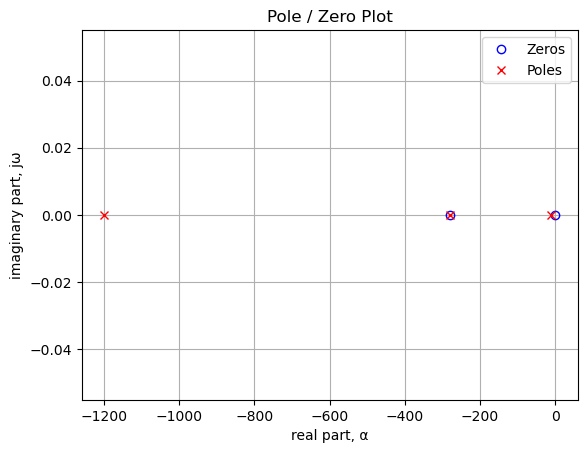

The code below generates a table that lists the values of the pole and zero locations.

table_header = ['Zeros, Hz', 'Poles, Hz']
num_table_rows = max(len(sys_zeros),len(sys_poles))
table_row = []

for i in range(num_table_rows):
    if i < len(sys_zeros):
        z = '{:.2f}'.format(sys_zeros[i]/(2*np.pi))
    else:
        z = ''
    if i < len(sys_poles):
        p = '{:.2f}'.format(sys_poles[i]/(2*np.pi))
    else:
        p = ''
    table_row.append([z,p])

print(tabulate(table_row, headers=table_header,colalign = ('left','left'),tablefmt="simple"))

Zeros, Hz    Poles, Hz
-----------  -----------
-280.86      -1198.55
0.00         -279.87
             -12.02

39.3.1.6 Reactive Branch 1 Frequency Response

The transfer function \(H(s)=\frac{v2}{v1}\) is analyzed for various settings of the Gain control, P1. The gain setting is in steps of percentage of full scale, from 1 to 99% and is plotted below.

# setup
x_axis = np.logspace(0, 5, 2000, endpoint=True)*2*np.pi
color_list = ['tab:blue','tab:purple','tab:brown','tab:red','tab:green','tab:orange','k']
gain_setting = np.array([1,2.5,9.75,25,50,75,99])/100
p1_value = 100e3

# plot
fig, ax1 = plt.subplots()
ax1.set_ylabel('magnitude, dB')
ax1.set_xlabel('frequency, Hz')

# instantiate a second y-axes that shares the same x-axis
ax2 = ax1.twinx()
color = 'k'

ax2.set_ylabel('phase, deg',color=color)
ax2.tick_params(axis='y', labelcolor=color)

for i in range(len(gain_setting)):
    element_values[Rp1b] = p1_value - gain_setting[i]*p1_value
    
    NE = NE_sym.subs(element_values)
    U = solve(NE,X)
    H = U[v2]/U[v1] #U[v2]/U[v1]
    num, denom = fraction(H) #returns numerator and denominator

    # convert symbolic to NumPy polynomial
    a = np.array(Poly(num, s).all_coeffs(), dtype=float)
    b = np.array(Poly(denom, s).all_coeffs(), dtype=float)
    sys = (a, b)

    #x = np.logspace(1, 5, 2000, endpoint=False)*2*np.pi
    w, mag, phase = signal.bode(sys, w=x_axis) # returns: rad/s, mag in dB, phase in deg

    # plot the results.  
    ax1.semilogx(w/(2*np.pi), mag,'-',color=color_list[i],label='magnitude @ {:.0f}% gain'.format(gain_setting[i]*100)) # magnitude plot
    ax2.semilogx(w/(2*np.pi), phase,':',color=color_list[i],label='phase @ {:.0f}% gain'.format(gain_setting[i]*100)) # phase plot

# highlight the guitar audio band, 80 to 8kHz
plt.axvspan(80, 8e3, color='y', alpha=0.3) 

# set plot limits for display
plt.xlim((1,100e3))
ax1.set_ylim((-60,10))

# position legends outside the graph
ax1.legend(bbox_to_anchor=(1.6,1)) # magnitude legend position: relative (horizontal position, vertical position) 
ax2.legend(bbox_to_anchor=(1.6,0.5)) # phase legend position:

ax1.grid()
plt.title('Magnitude and phase response for gains of 1% to 99%')
plt.show()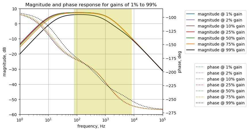

The plot above shows the band pass characteristic of the circuit in Figure 39.1. The highlighted frequencies are the guitar audio band. Rotation of \(P_{1B}\) has a limited effect in this path. Keep in mind that a pole at 500 Hz from \(C_{13}\) is not included which would move the low pass corner frequency considerably lower if it was included.

39.3.2 Reactive Branch 2

The circuit shown below is reactive branch 2. This circuit is part of the circuit path analyzed in Section 37.11.3 and is a slightly modified version of the highlighted portion of circuit shown in Figure 37.19.

Figure 39.2: Schematic of reactive branch 2.

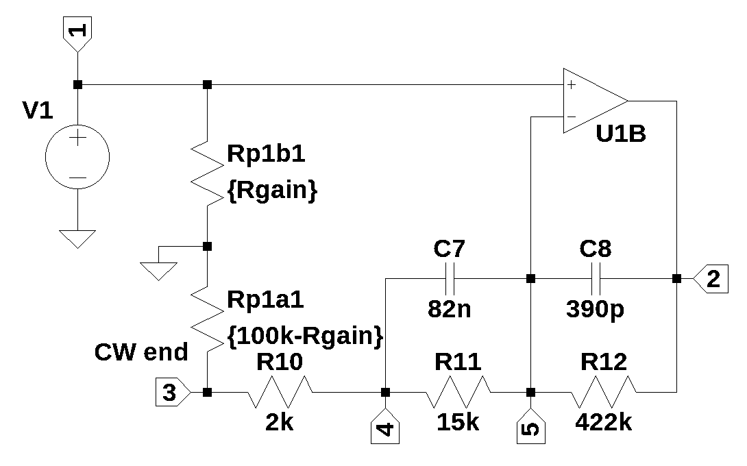
The schematic above includes the components that are in the feed back loop around U1B. \(P_1\) is modeled by two resistors, Rp1a1 and Rp1b1. The wiper of P1 is connected to ground. When \(P_1\) fully clockwise, \(V_1\) is shunted by the full value of \(P_1\), which is 100 k\(\Omega\), and node 3 is effectively connected to ground. When \(P_1\) is fully counter clockwise, the wiper, which is connected to ground is effectively grounding \(V_1\) and the non-inverting terminal of \(U_{1B}\), which prevents the signal from propagating to \(U_{1B}\).

The parallel combination of \(C_8\) and \(R_{12}\) along with \(C_7\) and \(R_{11}\) determine the frequency response. The netlist below was exported from LTSpice.

reactive_branch_2_net_list = '''
*reactive_branch_2.asc
V1 1 0 1
Rp1b1 0 1 50e3
Rp1a1 3 0 50e3
R10 4 3 2e3
R11 5 4 15e3
C7 5 4 82e-9
C8 2 5 390e-12
R12 2 5 422e3
O1B 5 1 2
'''

Using the function SymMNA.smna generate the network equations from the MNA matrices and display the equations.

report, network_df, i_unk_df, A, X, Z = SymMNA.smna(reactive_branch_2_net_list)

# Put matrices into SymPy 
X = Matrix(X)
Z = Matrix(Z)

NE_sym = Eq(A*X,Z)

# display the equations
temp = ''
for i in range(shape(NE_sym.lhs)[0]):
    temp += '${:s} = {:s}$<br>'.format(latex(NE_sym.rhs[i]),latex(NE_sym.lhs[i]))
Markdown(temp)

\(0 = I_{V1} + \frac{v_{1}}{Rp1b1}\)
\(0 = I_{O1b} + v_{2} \left(C_{8} s + \frac{1}{R_{12}}\right) + v_{5} \left(- C_{8} s - \frac{1}{R_{12}}\right)\)
\(0 = v_{3} \cdot \left(\frac{1}{Rp1a1} + \frac{1}{R_{10}}\right) - \frac{v_{4}}{R_{10}}\)
\(0 = v_{4} \left(C_{7} s + \frac{1}{R_{11}} + \frac{1}{R_{10}}\right) + v_{5} \left(- C_{7} s - \frac{1}{R_{11}}\right) - \frac{v_{3}}{R_{10}}\)
\(0 = v_{2} \left(- C_{8} s - \frac{1}{R_{12}}\right) + v_{4} \left(- C_{7} s - \frac{1}{R_{11}}\right) + v_{5} \left(C_{7} s + C_{8} s + \frac{1}{R_{12}} + \frac{1}{R_{11}}\right)\)
\(V_{1} = v_{1}\)
\(0 = - v_{1} + v_{5}\)

Turn the free symbols into SymPy variables and load the element values.

var(str(NE_sym.free_symbols).replace('{','').replace('}',''))
element_values = SymMNA.get_part_values(network_df)

39.3.2.1 Symbolic solution

The network equations for the circuit in Figure 39.2 can be solved symbolically.

U_sym = solve(NE_sym,X)

Display the symbolic solution.

temp = ''
for i in U_sym.keys():
    temp += '${:s} = {:s}$<br>'.format(latex(i),latex(U_sym[i]))

Markdown(temp)

\(v_{1} = V_{1}\)
\(v_{2} = \frac{C_{7} C_{8} R_{10} R_{11} R_{12} V_{1} s^{2} + C_{7} C_{8} R_{11} R_{12} Rp1a1 V_{1} s^{2} + C_{7} R_{10} R_{11} V_{1} s + C_{7} R_{11} R_{12} V_{1} s + C_{7} R_{11} Rp1a1 V_{1} s + C_{8} R_{10} R_{12} V_{1} s + C_{8} R_{11} R_{12} V_{1} s + C_{8} R_{12} Rp1a1 V_{1} s + R_{10} V_{1} + R_{11} V_{1} + R_{12} V_{1} + Rp1a1 V_{1}}{C_{7} C_{8} R_{10} R_{11} R_{12} s^{2} + C_{7} C_{8} R_{11} R_{12} Rp1a1 s^{2} + C_{7} R_{10} R_{11} s + C_{7} R_{11} Rp1a1 s + C_{8} R_{10} R_{12} s + C_{8} R_{11} R_{12} s + C_{8} R_{12} Rp1a1 s + R_{10} + R_{11} + Rp1a1}\)
\(v_{3} = \frac{C_{7} R_{11} Rp1a1 V_{1} s + Rp1a1 V_{1}}{C_{7} R_{10} R_{11} s + C_{7} R_{11} Rp1a1 s + R_{10} + R_{11} + Rp1a1}\)
\(v_{4} = \frac{C_{7} R_{10} R_{11} V_{1} s + C_{7} R_{11} Rp1a1 V_{1} s + R_{10} V_{1} + Rp1a1 V_{1}}{C_{7} R_{10} R_{11} s + C_{7} R_{11} Rp1a1 s + R_{10} + R_{11} + Rp1a1}\)
\(v_{5} = V_{1}\)
\(I_{V1} = - \frac{V_{1}}{Rp1b1}\)
\(I_{O1b} = \frac{- C_{7} R_{11} V_{1} s - V_{1}}{C_{7} R_{10} R_{11} s + C_{7} R_{11} Rp1a1 s + R_{10} + R_{11} + Rp1a1}\)

The network transfer function, \(H(s)=\frac {v_2(s)}{v_1(s)}\) is:

H_sym = (U_sym[v2]/U_sym[v1]).cancel()
Markdown('$H(s)={:s}$'.format(latex(H_sym)))

\(H(s)=\frac{C_{7} C_{8} R_{10} R_{11} R_{12} s^{2} + C_{7} C_{8} R_{11} R_{12} Rp1a1 s^{2} + C_{7} R_{10} R_{11} s + C_{7} R_{11} R_{12} s + C_{7} R_{11} Rp1a1 s + C_{8} R_{10} R_{12} s + C_{8} R_{11} R_{12} s + C_{8} R_{12} Rp1a1 s + R_{10} + R_{11} + R_{12} + Rp1a1}{C_{7} C_{8} R_{10} R_{11} R_{12} s^{2} + C_{7} C_{8} R_{11} R_{12} Rp1a1 s^{2} + C_{7} R_{10} R_{11} s + C_{7} R_{11} Rp1a1 s + C_{8} R_{10} R_{12} s + C_{8} R_{11} R_{12} s + C_{8} R_{12} Rp1a1 s + R_{10} + R_{11} + Rp1a1}\)

Both the numerator and denominator are second order polynomials.

H_sym_num, H_sym_denom = fraction(H_sym,s) #returns numerator and denominator

39.3.2.2 Numerator Polynomial

The numerator polynomial is:

Markdown('$N(s)={:s}$'.format(latex(H_sym_num)))

\(N(s)=C_{7} C_{8} R_{10} R_{11} R_{12} s^{2} + C_{7} C_{8} R_{11} R_{12} Rp1a1 s^{2} + C_{7} R_{10} R_{11} s + C_{7} R_{11} R_{12} s + C_{7} R_{11} Rp1a1 s + C_{8} R_{10} R_{12} s + C_{8} R_{11} R_{12} s + C_{8} R_{12} Rp1a1 s + R_{10} + R_{11} + R_{12} + Rp1a1\)

The coefficients of each Laplace term can be equated to the variables \(b_2\), \(b_1\) and \(b_0\) in the expression:

\(b_2s^{2}+b_1s+b_0\)

where \(b_2\), \(b_1\) and \(b_0\) are:

b2 = H_sym_num.coeff(s**2)
b1 = H_sym_num.coeff(s**1)
b0 = (H_sym_num - b1*s*1 - b2*s**2).expand()

Markdown('<p>$b_2={:s}$</p><p>$b_1={:s}$\
    </p><p>$b_0={:s}$</p>'.format(latex(b2),latex(b1),latex(b0)))

\(b_2=C_{7} C_{8} R_{10} R_{11} R_{12} + C_{7} C_{8} R_{11} R_{12} Rp1a1\)

\(b_1=C_{7} R_{10} R_{11} + C_{7} R_{11} R_{12} + C_{7} R_{11} Rp1a1 + C_{8} R_{10} R_{12} + C_{8} R_{11} R_{12} + C_{8} R_{12} Rp1a1\)

\(b_0=R_{10} + R_{11} + R_{12} + Rp1a1\)

The roots of the numerator polynomial can easily be found with SymPy. This filter has two transmission zeros, which can be found using the solve function on the numerator polynomial.

num_root_sym = solve(H_sym_num,s)

Markdown('There are {:d} zeros, which are:\
    <p>$z_0={:s}$</p><p>$z_1={:s}$</p>'.format(len(num_root_sym),latex(num_root_sym[0]),latex(num_root_sym[1])))

There are 2 zeros, which are:

\(z_0=\frac{- C_{7} R_{10} R_{11} - C_{7} R_{11} R_{12} - C_{7} R_{11} Rp1a1 - C_{8} R_{10} R_{12} - C_{8} R_{11} R_{12} - C_{8} R_{12} Rp1a1 - \sqrt{C_{7}^{2} R_{10}^{2} R_{11}^{2} + 2 C_{7}^{2} R_{10} R_{11}^{2} R_{12} + 2 C_{7}^{2} R_{10} R_{11}^{2} Rp1a1 + C_{7}^{2} R_{11}^{2} R_{12}^{2} + 2 C_{7}^{2} R_{11}^{2} R_{12} Rp1a1 + C_{7}^{2} R_{11}^{2} Rp1a1^{2} - 2 C_{7} C_{8} R_{10}^{2} R_{11} R_{12} - 2 C_{7} C_{8} R_{10} R_{11}^{2} R_{12} - 2 C_{7} C_{8} R_{10} R_{11} R_{12}^{2} - 4 C_{7} C_{8} R_{10} R_{11} R_{12} Rp1a1 + 2 C_{7} C_{8} R_{11}^{2} R_{12}^{2} - 2 C_{7} C_{8} R_{11}^{2} R_{12} Rp1a1 - 2 C_{7} C_{8} R_{11} R_{12}^{2} Rp1a1 - 2 C_{7} C_{8} R_{11} R_{12} Rp1a1^{2} + C_{8}^{2} R_{10}^{2} R_{12}^{2} + 2 C_{8}^{2} R_{10} R_{11} R_{12}^{2} + 2 C_{8}^{2} R_{10} R_{12}^{2} Rp1a1 + C_{8}^{2} R_{11}^{2} R_{12}^{2} + 2 C_{8}^{2} R_{11} R_{12}^{2} Rp1a1 + C_{8}^{2} R_{12}^{2} Rp1a1^{2}}}{2 C_{7} C_{8} R_{11} R_{12} \left(R_{10} + Rp1a1\right)}\)

\(z_1=\frac{- C_{7} R_{10} R_{11} - C_{7} R_{11} R_{12} - C_{7} R_{11} Rp1a1 - C_{8} R_{10} R_{12} - C_{8} R_{11} R_{12} - C_{8} R_{12} Rp1a1 + \sqrt{C_{7}^{2} R_{10}^{2} R_{11}^{2} + 2 C_{7}^{2} R_{10} R_{11}^{2} R_{12} + 2 C_{7}^{2} R_{10} R_{11}^{2} Rp1a1 + C_{7}^{2} R_{11}^{2} R_{12}^{2} + 2 C_{7}^{2} R_{11}^{2} R_{12} Rp1a1 + C_{7}^{2} R_{11}^{2} Rp1a1^{2} - 2 C_{7} C_{8} R_{10}^{2} R_{11} R_{12} - 2 C_{7} C_{8} R_{10} R_{11}^{2} R_{12} - 2 C_{7} C_{8} R_{10} R_{11} R_{12}^{2} - 4 C_{7} C_{8} R_{10} R_{11} R_{12} Rp1a1 + 2 C_{7} C_{8} R_{11}^{2} R_{12}^{2} - 2 C_{7} C_{8} R_{11}^{2} R_{12} Rp1a1 - 2 C_{7} C_{8} R_{11} R_{12}^{2} Rp1a1 - 2 C_{7} C_{8} R_{11} R_{12} Rp1a1^{2} + C_{8}^{2} R_{10}^{2} R_{12}^{2} + 2 C_{8}^{2} R_{10} R_{11} R_{12}^{2} + 2 C_{8}^{2} R_{10} R_{12}^{2} Rp1a1 + C_{8}^{2} R_{11}^{2} R_{12}^{2} + 2 C_{8}^{2} R_{11} R_{12}^{2} Rp1a1 + C_{8}^{2} R_{12}^{2} Rp1a1^{2}}}{2 C_{7} C_{8} R_{11} R_{12} \left(R_{10} + Rp1a1\right)}\)

39.3.2.3 Denominator Polynomial

The denominator polynomial is:

Markdown('$D(s)={:s}$'.format(latex(H_sym_denom)))

\(D(s)=C_{7} C_{8} R_{10} R_{11} R_{12} s^{2} + C_{7} C_{8} R_{11} R_{12} Rp1a1 s^{2} + C_{7} R_{10} R_{11} s + C_{7} R_{11} Rp1a1 s + C_{8} R_{10} R_{12} s + C_{8} R_{11} R_{12} s + C_{8} R_{12} Rp1a1 s + R_{10} + R_{11} + Rp1a1\)

The coefficients of each Laplace term can be equated to the variables \(a_3\), \(a_2\), \(a_1\) and \(a_0\) in the expression:

\(a_3s^3+a_2s^2+a_1s+a_0\)

where \(a_3\), \(a_2\), \(a_1\) and \(a_0\) are:

\(a_2=C_{7} C_{8} R_{10} R_{11} R_{12} + C_{7} C_{8} R_{11} R_{12} Rp1a1\)

\(a_1=C_{7} R_{10} R_{11} + C_{7} R_{11} Rp1a1 + C_{8} R_{10} R_{12} + C_{8} R_{11} R_{12} + C_{8} R_{12} Rp1a1\)

\(a_0=R_{10} + R_{11} + Rp1a1\)

The roots of the denominator polynomial can be found with SymPy.

denom_root_sym = solve(H_sym_denom,s)

Markdown('There are {:d} poles, which are:\
    <p>$p_0={:s}$</p><p>$p_1={:s}$</p>'.format(len(denom_root_sym),latex(denom_root_sym[0]),latex(denom_root_sym[1])))

There are 2 poles, which are:

\(p_0=- \frac{1}{C_{8} R_{12}}\)

\(p_1=\frac{- R_{10} - R_{11} - Rp1a1}{C_{7} R_{11} \left(R_{10} + Rp1a1\right)}\)

39.3.2.4 Numerical Solution for P1 at 50%

A numerical solution for the network equations is obtained for P1 at 50% rotation. The element values are substituted into the equations and displayed.

equ_N = NE_sym.subs(element_values)

temp = ''
for i in range(shape(equ_N.lhs)[0]):
    temp += '<p>${:s} = {:s}$</p>'.format(latex(equ_N.rhs[i]),
        latex(round_expr(equ_N.lhs[i],6)))

Markdown(temp)

\(0 = I_{V1} + 2.0 \cdot 10^{-5} v_{1}\)

\(0 = I_{O1b} + 2.0 \cdot 10^{-6} v_{2} - 2.0 \cdot 10^{-6} v_{5}\)

\(0 = 0.00052 v_{3} - 0.0005 v_{4}\)

\(0 = - 0.0005 v_{3} + 0.000567 v_{4} - 6.7 \cdot 10^{-5} v_{5}\)

\(0 = - 2.0 \cdot 10^{-6} v_{2} - 6.7 \cdot 10^{-5} v_{4} + 6.9 \cdot 10^{-5} v_{5}\)

\(1.0 = v_{1}\)

\(0 = - v_{1} + v_{5}\)

SymPy can solve for unknown node voltages and the unknown currents from the independent voltage source, \(V_1\), and the Op Amp’s output terminal. The unknown currents, \(I_{V1}\) and \(I_{O1}\), are not displayed. The node voltages are:

U = solve(equ_N,X)

temp = ''
for i in U.keys():
    if str(i)[0] == 'v': # only display the node voltages
        temp += '<p>${:s} = {:s}$</p>'.format(latex(i),latex(U[i]))

Markdown(temp)

\(v_{1} = 1.0\)

\(v_{2} = \frac{3.74166 \cdot 10^{22} s^{2} + 2.11154097156402 \cdot 10^{27} s + 1.7381516587678 \cdot 10^{30}}{3.74166 \cdot 10^{22} s^{2} + 2.66540971563981 \cdot 10^{26} s + 2.38151658767774 \cdot 10^{29}}\)

\(v_{3} = \frac{3075000000000.0 s + 2.5 \cdot 10^{15}}{3198000000000.0 s + 3.35000000000001 \cdot 10^{15}}\)

\(v_{4} = \frac{3198000000000.0 s + 2.6 \cdot 10^{15}}{3198000000000.0 s + 3.35000000000001 \cdot 10^{15}}\)

\(v_{5} = 1.0\)

The network transfer function, \(H(s)=\frac {v_2(s)}{v_1(s)}\), is:

H = (U[v2]/U[v1]).cancel()
Markdown('$H(s)={:s}$'.format(latex(H)))

\(H(s)=\frac{3.74166 \cdot 10^{22} s^{2} + 2.11154097156402 \cdot 10^{27} s + 1.7381516587678 \cdot 10^{30}}{3.74166 \cdot 10^{22} s^{2} + 2.66540971563981 \cdot 10^{26} s + 2.38151658767774 \cdot 10^{29}}\)

The SciPy function, TransferFunction, is used to represent the system as the continuous-time transfer function. The code below extracts the numerator and denominator polynomials from the voltage transfer function. Then coefficients of the terms are used to build a SciPy transfer function object.

H_num, H_denom = fraction(H) #returns numerator and denominator

# convert symbolic to NumPy polynomial
a = np.array(Poly(H_num, s).all_coeffs(), dtype=float)
b = np.array(Poly(H_denom, s).all_coeffs(), dtype=float)

sys_tf = signal.TransferFunction(a,b)

39.3.2.5 Pole Zero Plot

The poles and zeros of the transfer function can easily be obtained with the following code:

sys_zeros = np.roots(sys_tf.num)
sys_poles = np.roots(sys_tf.den)

The poles and zeros of the transfer function are plotted on the complex frequency plane with the following code:

plt.plot(np.real(sys_zeros/(2*np.pi)), np.imag(sys_zeros/(2*np.pi)), 'ob',
    markerfacecolor='none')
plt.plot(np.real(sys_poles/(2*np.pi)), np.imag(sys_poles/(2*np.pi)), 'xr')
plt.legend(['Zeros', 'Poles'], loc=0)
plt.title('Pole / Zero Plot')
plt.xlabel('real part, \u03B1')
plt.ylabel('imaginary part, j\u03C9')
plt.grid()
plt.show()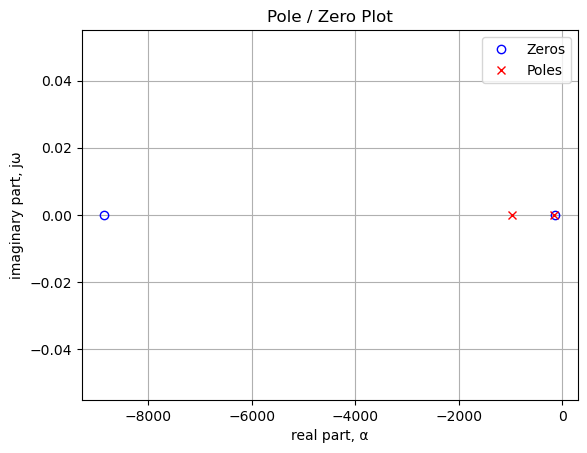

The code below generates a table that lists the values of the pole and zero locations.

table_header = ['Zeros, Hz', 'Poles, Hz']
num_table_rows = max(len(sys_zeros),len(sys_poles))
table_row = []

for i in range(num_table_rows):
    if i < len(sys_zeros):
        z = '{:.2f}'.format(sys_zeros[i]/(2*np.pi))
    else:
        z = ''
    if i < len(sys_poles):
        p = '{:.2f}'.format(sys_poles[i]/(2*np.pi))
    else:
        p = ''
    table_row.append([z,p])

print(tabulate(table_row, headers=table_header,colalign = ('left','left'),tablefmt="simple"))

Zeros, Hz    Poles, Hz
-----------  -----------
-8848.65     -967.04
-132.98      -166.72

39.3.2.6 Pole/Zero Locus Plot versus \(P_1\) value

For each position of \(P_1\), there are two zeros and two poles. The plot below shows the frequency locations for the pole and zero locations as a function of \(P_1\) rotation. Since the poles and zeros don’t have imaginary parts, the complex frequency is plotted on the vertical axis versus the gain control rotational position, from 1 to 99 percent. The plot provides a visual indication of how the poles and zeros change as a function \(P_1\).

sym_num, sym_denom = fraction(H_sym) #returns numerator and denominator

p1_value = 100e3
num_roots = []
denom_roots = []
for i in np.linspace(1,99,20)/100:
    element_values[Rp1a1] = p1_value - i*p1_value
    element_values[Rp1b1] = i*p1_value
    num_roots.append(solve(sym_num.subs(element_values),s))
    denom_roots.append(solve(sym_denom.subs(element_values),s))

# put the zeros into an array
z0_locus = np.zeros(len(np.array(num_roots)))
z1_locus = np.zeros(len(np.array(num_roots)))
for i in range(len(np.array(num_roots))):
    z0_locus[i] = -np.array(num_roots)[i][0]    
    z1_locus[i] = -np.array(num_roots)[i][1]        

# put the poles into an array
p0_locus = np.zeros(len(np.array(denom_roots)))
p1_locus = np.zeros(len(np.array(denom_roots)))
for i in range(len(np.array(denom_roots))):
    p0_locus[i] = -np.array(denom_roots)[i][0]    
    p1_locus[i] = -np.array(denom_roots)[i][1]        

After solving for the numerator and dominator roots of the transfer function at various positions of \(P_1\), we can examine the range of frequencies that the zeros take on as \(P_1\) is rotated.

print(f'z0 range as a function of P1: {z0_locus.min()/(2*np.pi)/1e3:.3f} to {z0_locus.max()/(2*np.pi)/1e3:.3f} kHz')
print(f'z1 range as a function of P1: {z1_locus.min()/(2*np.pi)/1e3:.3f} to {z1_locus.max()/(2*np.pi)/1e3:.3f} kHz')

z0 range as a function of P1: 5.023 to 137.640 kHz
z1 range as a function of P1: 0.133 to 0.133 kHz

As shown above, \(z_0\) will move from about 5kHz to 137 kHz as \(P_1\) is rotated. \(z_1\)’s position in the complex frequency plane remains constant. The position of \(z_0\) is plotted below.

plt.plot(np.linspace(1,99,len(np.array(num_roots))),z0_locus/(2*np.pi)/1e3,'o-b', markerfacecolor='none',label='z_0')
#plt.plot(np.linspace(1,99,len(np.array(num_roots))),z1_locus/(2*np.pi)/1e3,'o-b', markerfacecolor='none',label='z_1')

#plt.plot(np.linspace(1,99,len(np.array(denom_roots))),p0_locus/(2*np.pi)/1e3,'x-r', markerfacecolor='none',label='p_0')
#plt.plot(np.linspace(1,99,len(np.array(denom_roots))),p1_locus/(2*np.pi)/1e3,'x-r', markerfacecolor='none',label='p_1')

plt.ylim((0,140))
plt.legend(loc='upper left')
plt.title('Gain control pole & zero frequency plot vs gain rotation %')
plt.xlabel('Gain rotation percentage')
plt.ylabel('pole and zero frequency, kHz')
plt.grid()

plt.show()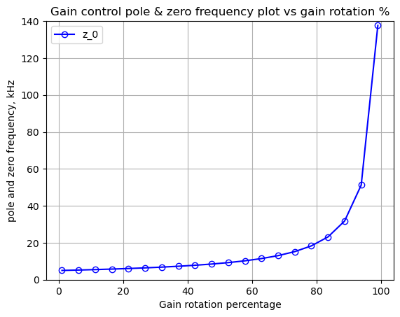

As shown above, the position of \(z_0\) moves more dramatically when \(P_1\) is rotated from 80 to 100%.

The range of the poles on the complex plane is printed below.

print(f'p0 range as a function of P1: {p0_locus.min()/(2*np.pi)/1e3:.3f} to {p0_locus.max()/(2*np.pi)/1e3:.3f} kHz')
print(f'p1 range as a function of P1: {p1_locus.min()/(2*np.pi)/1e3:.3f} to {p1_locus.max()/(2*np.pi)/1e3:.3f} kHz')

p0 range as a function of P1: 0.967 to 0.967 kHz
p1 range as a function of P1: 0.149 to 0.776 kHz

The position of \(p_0\) is constant and \(p_1\) moves from 150 Hz to 776 Hz as \(P_1\) is rotated.

#plt.plot(np.linspace(1,99,len(np.array(num_roots))),z0_locus/(2*np.pi)/1e3,'o-b', markerfacecolor='none',label='z_0')
#plt.plot(np.linspace(1,99,len(np.array(num_roots))),z1_locus/(2*np.pi)/1e3,'o-b', markerfacecolor='none',label='z_1')

#plt.plot(np.linspace(1,99,len(np.array(denom_roots))),p0_locus/(2*np.pi)/1e3,'x-k', markerfacecolor='none',label='p_0')
plt.plot(np.linspace(1,99,len(np.array(denom_roots))),p1_locus/(2*np.pi)/1e3,'x-r', markerfacecolor='none',label='p_1')

plt.ylim((0,1))
plt.legend(loc='upper left')
plt.title('Gain control pole & zero frequency plot vs gain rotation %')
plt.xlabel('Gain rotation percentage')
plt.ylabel('pole and zero frequency, kHz')
plt.grid()

plt.show()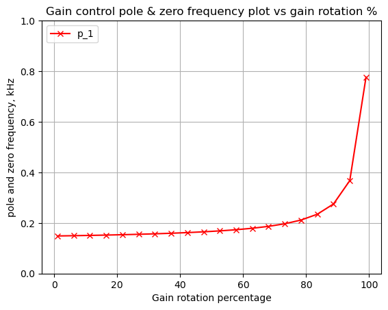

As shown above, \(p_1\) moves more dramatically as \(P_1\) is rotated from 80% to 100%.

39.3.2.7 Reactive Branch 2 Frequency Response

The voltage transfer function for the reactive branch shown in Figure 39.2 is plotted below.

# set up
x_axis = np.logspace(1, 5, 2000, endpoint=False)*2*np.pi
color_list = ['tab:blue','tab:red','tab:green','tab:orange','k']
gain_setting = np.array([1,25,50,75,99])/100
p1_value = 100e3

# plot
fig, ax1 = plt.subplots()
ax1.set_ylabel('magnitude, dB')
ax1.set_xlabel('frequency, Hz')

# instantiate a second y-axes that shares the same x-axis
ax2 = ax1.twinx()
color = 'k'

ax2.set_ylabel('phase, deg',color=color)
ax2.tick_params(axis='y', labelcolor=color)

for i in range(len(gain_setting)):
    element_values[Rp1a1] = p1_value - gain_setting[i]*p1_value
    element_values[Rp1b1] = gain_setting[i]*p1_value
    
    #element_values[Rp1a2] = p1_value - gain_setting[i]*p1_value
    #element_values[Rp1b2] = gain_setting[i]*p1_value
    
    NE = NE_sym.subs(element_values)
    U = solve(NE,X)
    H = U[v2]/U[v1]
    num, denom = fraction(H) #returns numerator and denominator

    # convert symbolic to NumPy polynomial
    a = np.array(Poly(num, s).all_coeffs(), dtype=float)
    b = np.array(Poly(denom, s).all_coeffs(), dtype=float)
    #tf_num_coef_list.append(a)
    #tf_denom_coef_list.append(b)
    
    #x = np.logspace(1, 5, 2000, endpoint=False)*2*np.pi
    w, mag, phase = signal.bode((a, b), w=x_axis) # returns: rad/s, mag in dB, phase in deg
    #clean_path1_mag[i] = mag
    
    # plot the results.  
    ax1.semilogx(w/(2*np.pi), mag,'-',color=color_list[i],label='mag: {:.0f}%'.format(gain_setting[i]*100))    # magnitude plot
    ax2.semilogx(w/(2*np.pi), phase,':',color=color_list[i],label='phase: {:.0f}%'.format(gain_setting[i]*100))  # phase plot

# highlight the guitar audio band, 80 to 8kHz
plt.axvspan(80, 8e3, color='y', alpha=0.3) 

# position legends outside the graph
ax1.legend(bbox_to_anchor=(1.6,1)) # magnitude legend position: relative (horizontal position, vertical position) 
ax2.legend(bbox_to_anchor=(1.6,0.5)) # phase legend position:

#ax1.legend(loc='lower left')
#ax2.legend(loc='lower right')
ax1.grid()
plt.title('Magnitude and phase response')
plt.show()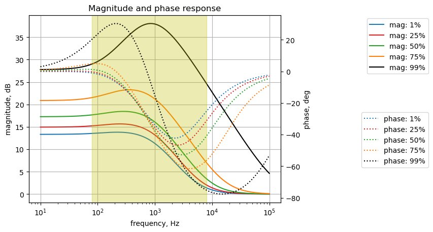

As shown above, when the gain is increased, a resonance develops near 1 kHz.

39.3.3 Reactive Branch 3

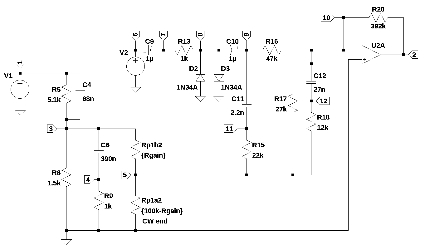
The schematic shown below represents the highlighted parts of the Klon Centuar circuit shown in Figure 37.17 and Figure 37.21. The voltage source \(V_1\) is the output Op Amp of \(U_{1A}\) and the voltage source \(V_2\) is the output of \(U_{1B}\). The Diodes \(D_1\) and \(D_2\) have been commented out in the netlist. Node 10 is the summing junction for clean path 2 and the diode path.

One of the ganged pots in \(P_1\), which is the gain control, is represented in the schematic by the resistors \(R_{p1b2}\) and \(R_{p1a2}\). The variable \(R_{gain}\) is used to control the position of the wiper. The gain pot, \(P_1\)’s terminals, are across \(R_9\) and \(C_6\) and \(P_1\)’s wiper contact at node 5 and forms a voltage divider that controls the signal amplitude at node 5.

In this section of the analysis we will look at the reactive path from node 1 to node 2 with \(V_2\) set to zero. This will include most of the components that are attached to these nodes. The components that are not included are those components along clean path 1 shown in Figure 37.15. Node 10 below is a virtual ground and by superposition we can separate out the contribution from clan path 1 and add it back later if we want to consider the combined contribution of the signals from the inputs to the summing junction. For now we are only interested in reactive branch 3.

The capacitor \(C_{13}\) shown in Figure 37.17 has been removed from this analysis. \(C_{13}\) in parallel with \(R_{20}\) in the feedback path around \(U_{2B}\) adds a zero to the voltage transfer function at about 500 Hz. The effect of this low pass filter is excluded from this analysis since we are interested only in the reactive path prior to \(U_{1B}\)

We will examine the solution to the network equations with \(P_1\) set to 50%. A symbolic solution was taking too long on my laptop, so this step was skipped. The poles and zeros for \(P_1\) are plotted and tabulated. The locus of poles and zeros for the transfer function are plotted to see how they move in the frequency domain as a function of \(P_1\). Finally, a frequency response plot of the voltage transfer function versus gain settings is generated.

In Section 39.3.4 and Section 39.3.6, reactive branch 3 is divided into two smaller subcircuits at \(P_1\). This is done to gain some insight into the operation of components along this path.

Figure 39.3: Schematic of reactive branches 3 and 4. Reactive branch 3 is the path from V1 to V2 and reactive branch 4 is the path from V3 to V2.

The netlist below was exported from LTSpice when the schematic was generated.

Reactive_branch_3_4_net_list = '''
* Reactive_branch_3&4.asc
V1 1 0 1
V2 6 0 0
R5 1 3 5.1e3
R8 3 0 1.5e3
C4 1 3 68e-9
C6 3 4 390e-9
R9 4 0 1e3
Rp1b2 3 5 50e3
Rp1a2 5 0 50e3
R13 8 7 1e3
C11 9 11 2.2e-9
R15 11 5 22e3
R17 10 5 27e3
R18 12 5 12e3
C12 10 12 27e-9
R16 10 9 47e3
*R20 2 10 100e3
R20 2 10 392e3
*C13 2 10 820e-12
O2a 10 0 2
*D2 0 8 1N34A
*D3 8 0 1N34A
C9 6 7 1e-6
C10 9 8 1e-6
'''

The function SymMNA.smna generates the MNA matrices from the netlist.

report, network_df, i_unk_df, A, X, Z = SymMNA.smna(Reactive_branch_3_4_net_list)

The following code builds and displays the symbolic circuit equations.

# Put matrices into SymPy 
X = Matrix(X)
Z = Matrix(Z)

NE_sym = Eq(A*X,Z)

# display the equations
temp = ''
for i in range(shape(NE_sym.lhs)[0]):
    temp += '${:s} = {:s}$<br>'.format(latex(NE_sym.rhs[i]),latex(NE_sym.lhs[i]))
Markdown(temp)

\(0 = I_{V1} + v_{1} \left(C_{4} s + \frac{1}{R_{5}}\right) + v_{3} \left(- C_{4} s - \frac{1}{R_{5}}\right)\)
\(0 = I_{O2a} - \frac{v_{10}}{R_{20}} + \frac{v_{2}}{R_{20}}\)
\(0 = - C_{6} s v_{4} + v_{1} \left(- C_{4} s - \frac{1}{R_{5}}\right) + v_{3} \left(C_{4} s + C_{6} s + \frac{1}{Rp1b2} + \frac{1}{R_{8}} + \frac{1}{R_{5}}\right) - \frac{v_{5}}{Rp1b2}\)
\(0 = - C_{6} s v_{3} + v_{4} \left(C_{6} s + \frac{1}{R_{9}}\right)\)
\(0 = v_{5} \cdot \left(\frac{1}{Rp1b2} + \frac{1}{Rp1a2} + \frac{1}{R_{18}} + \frac{1}{R_{17}} + \frac{1}{R_{15}}\right) - \frac{v_{3}}{Rp1b2} - \frac{v_{12}}{R_{18}} - \frac{v_{10}}{R_{17}} - \frac{v_{11}}{R_{15}}\)
\(0 = C_{9} s v_{6} - C_{9} s v_{7} + I_{V2}\)
\(0 = - C_{9} s v_{6} + v_{7} \left(C_{9} s + \frac{1}{R_{13}}\right) - \frac{v_{8}}{R_{13}}\)
\(0 = - C_{10} s v_{9} + v_{8} \left(C_{10} s + \frac{1}{R_{13}}\right) - \frac{v_{7}}{R_{13}}\)
\(0 = - C_{10} s v_{8} - C_{11} s v_{11} + v_{9} \left(C_{10} s + C_{11} s + \frac{1}{R_{16}}\right) - \frac{v_{10}}{R_{16}}\)
\(0 = - C_{12} s v_{12} + v_{10} \left(C_{12} s + \frac{1}{R_{20}} + \frac{1}{R_{17}} + \frac{1}{R_{16}}\right) - \frac{v_{2}}{R_{20}} - \frac{v_{5}}{R_{17}} - \frac{v_{9}}{R_{16}}\)
\(0 = - C_{11} s v_{9} + v_{11} \left(C_{11} s + \frac{1}{R_{15}}\right) - \frac{v_{5}}{R_{15}}\)
\(0 = - C_{12} s v_{10} + v_{12} \left(C_{12} s + \frac{1}{R_{18}}\right) - \frac{v_{5}}{R_{18}}\)
\(V_{1} = v_{1}\)
\(V_{2} = v_{6}\)
\(0 = v_{10}\)

The free symbols in the equations above are turned into SymPy variables and the element values are loaded into a Python dictionary.

var(str(NE_sym.free_symbols).replace('{','').replace('}',''))
element_values = SymMNA.get_part_values(network_df)

39.3.3.1 Numerical Solution for P1 at 50%

The network equations were too complex to generate symbolic solutions on my laptop. A numerical solution for the equations can easily be generated and this was done for \(P_1\) = 50%. The element values are substituted into the equations and displayed.

equ_N = NE_sym.subs(element_values)

temp = ''
for i in range(shape(equ_N.lhs)[0]):
    temp += '<p>${:s} = {:s}$</p>'.format(latex(equ_N.rhs[i]),
        latex(round_expr(equ_N.lhs[i],9)))

Markdown(temp)

\(0 = I_{V1} + v_{1} \cdot \left(6.8 \cdot 10^{-8} s + 0.000196078\right) + v_{3} \left(- 6.8 \cdot 10^{-8} s - 0.000196078\right)\)

\(0 = I_{O2a} - 2.551 \cdot 10^{-6} v_{10} + 2.551 \cdot 10^{-6} v_{2}\)

\(0 = - 3.9 \cdot 10^{-7} s v_{4} + v_{1} \left(- 6.8 \cdot 10^{-8} s - 0.000196078\right) + v_{3} \cdot \left(4.58 \cdot 10^{-7} s + 0.000882745\right) - 2.0 \cdot 10^{-5} v_{5}\)

\(0 = - 3.9 \cdot 10^{-7} s v_{3} + v_{4} \cdot \left(3.9 \cdot 10^{-7} s + 0.001\right)\)

\(0 = - 3.7037 \cdot 10^{-5} v_{10} - 4.5455 \cdot 10^{-5} v_{11} - 8.3333 \cdot 10^{-5} v_{12} - 2.0 \cdot 10^{-5} v_{3} + 0.000205825 v_{5}\)

\(0 = I_{V2} + 1.0 \cdot 10^{-6} s v_{6} - 1.0 \cdot 10^{-6} s v_{7}\)

\(0 = - 1.0 \cdot 10^{-6} s v_{6} + v_{7} \cdot \left(1.0 \cdot 10^{-6} s + 0.001\right) - 0.001 v_{8}\)

\(0 = - 1.0 \cdot 10^{-6} s v_{9} - 0.001 v_{7} + v_{8} \cdot \left(1.0 \cdot 10^{-6} s + 0.001\right)\)

\(0 = - 2.0 \cdot 10^{-9} s v_{11} - 1.0 \cdot 10^{-6} s v_{8} - 2.1277 \cdot 10^{-5} v_{10} + v_{9} \cdot \left(1.002 \cdot 10^{-6} s + 2.1277 \cdot 10^{-5}\right)\)

\(0 = - 2.7 \cdot 10^{-8} s v_{12} + v_{10} \cdot \left(2.7 \cdot 10^{-8} s + 6.0865 \cdot 10^{-5}\right) - 2.551 \cdot 10^{-6} v_{2} - 3.7037 \cdot 10^{-5} v_{5} - 2.1277 \cdot 10^{-5} v_{9}\)

\(0 = - 2.0 \cdot 10^{-9} s v_{9} + v_{11} \cdot \left(2.0 \cdot 10^{-9} s + 4.5455 \cdot 10^{-5}\right) - 4.5455 \cdot 10^{-5} v_{5}\)

\(0 = - 2.7 \cdot 10^{-8} s v_{10} + v_{12} \cdot \left(2.7 \cdot 10^{-8} s + 8.3333 \cdot 10^{-5}\right) - 8.3333 \cdot 10^{-5} v_{5}\)

\(1.0 = v_{1}\)

\(0 = v_{6}\)

\(0 = v_{10}\)

Use SymPy to solve for the unknown voltages and currents in the network equations. The unknown currents, \(I_{V1}\) and \(I_{O1}\), are not displayed. The node voltages are:

U = solve(equ_N,X)

temp = ''
for i in U.keys():
    if str(i)[0] == 'v': # only display the node voltages
        temp += '<p>${:s} = {:s}$</p>'.format(latex(i),latex(U[i]))

Markdown(temp)

\(v_{1} = 1.0\)

\(v_{2} = \frac{- 2.02215504303191 \cdot 10^{56} s^{5} - 5.2950674540929 \cdot 10^{60} s^{4} - 2.8308370994823 \cdot 10^{64} s^{3} - 5.27827462462547 \cdot 10^{67} s^{2} - 3.01998947548071 \cdot 10^{70} s - 1.16148974096409 \cdot 10^{72}}{4.3362244543883 \cdot 10^{55} s^{5} + 2.06897279791109 \cdot 10^{60} s^{4} + 2.53915433684715 \cdot 10^{64} s^{3} + 5.64733157523515 \cdot 10^{67} s^{2} + 3.55388545376323 \cdot 10^{70} s + 1.37913277012933 \cdot 10^{72}}\)

\(v_{3} = \frac{7.70884347446809 \cdot 10^{55} s^{5} + 1.76830244412326 \cdot 10^{60} s^{4} + 9.75686883763291 \cdot 10^{63} s^{3} + 2.00756023341467 \cdot 10^{67} s^{2} + 1.40196836955285 \cdot 10^{70} s + 5.47822825670137 \cdot 10^{71}}{7.70884347446809 \cdot 10^{55} s^{5} + 3.67817386295305 \cdot 10^{60} s^{4} + 4.51405215439493 \cdot 10^{64} s^{3} + 1.00397005781958 \cdot 10^{68} s^{2} + 6.31801858446797 \cdot 10^{70} s + 2.45179159134104 \cdot 10^{72}}\)

\(v_{4} = \frac{7.70884347446809 \cdot 10^{55} s^{5} + 1.57063979093177 \cdot 10^{60} s^{4} + 5.72958732242324 \cdot 10^{63} s^{3} + 5.3843527894717 \cdot 10^{66} s^{2} + 2.13650902011353 \cdot 10^{68} s}{7.70884347446809 \cdot 10^{55} s^{5} + 3.67817386295305 \cdot 10^{60} s^{4} + 4.51405215439493 \cdot 10^{64} s^{3} + 1.00397005781958 \cdot 10^{68} s^{2} + 6.31801858446797 \cdot 10^{70} s + 2.45179159134104 \cdot 10^{72}}\)

\(v_{5} = \frac{4.72614965425532 \cdot 10^{53} s^{5} + 1.34411248109 \cdot 10^{58} s^{4} + 9.21167841492205 \cdot 10^{61} s^{3} + 2.41846205484128 \cdot 10^{65} s^{2} + 2.24113593696666 \cdot 10^{68} s + 8.88895209921494 \cdot 10^{69}}{4.81802717154256 \cdot 10^{54} s^{5} + 2.29885866434566 \cdot 10^{59} s^{4} + 2.82128259649683 \cdot 10^{63} s^{3} + 6.27481286137239 \cdot 10^{66} s^{2} + 3.94876161529248 \cdot 10^{69} s + 1.53236974458815 \cdot 10^{71}}\)

\(v_{6} = 0.0\)

\(v_{7} = \frac{2.0138625 \cdot 10^{55} s^{4} + 1.71863602941176 \cdot 10^{59} s^{3} + 4.87499999999999 \cdot 10^{62} s^{2} + 4.59558823529411 \cdot 10^{65} s}{4.81802717154256 \cdot 10^{54} s^{5} + 2.29885866434566 \cdot 10^{59} s^{4} + 2.82128259649683 \cdot 10^{63} s^{3} + 6.27481286137239 \cdot 10^{66} s^{2} + 3.94876161529248 \cdot 10^{69} s + 1.53236974458815 \cdot 10^{71}}\)

\(v_{8} = \frac{2.0138625 \cdot 10^{52} s^{5} + 1.92002227941176 \cdot 10^{56} s^{4} + 6.59363602941176 \cdot 10^{59} s^{3} + 9.47058823529411 \cdot 10^{62} s^{2} + 4.59558823529411 \cdot 10^{65} s}{4.81802717154256 \cdot 10^{54} s^{5} + 2.29885866434566 \cdot 10^{59} s^{4} + 2.82128259649683 \cdot 10^{63} s^{3} + 6.27481286137239 \cdot 10^{66} s^{2} + 3.94876161529248 \cdot 10^{69} s + 1.53236974458815 \cdot 10^{71}}\)

\(v_{9} = \frac{2.0138625 \cdot 10^{52} s^{5} + 2.12140852941176 \cdot 10^{56} s^{4} + 8.31227205882352 \cdot 10^{59} s^{3} + 1.43455882352941 \cdot 10^{63} s^{2} + 9.19117647058822 \cdot 10^{65} s}{4.81802717154256 \cdot 10^{54} s^{5} + 2.29885866434566 \cdot 10^{59} s^{4} + 2.82128259649683 \cdot 10^{63} s^{3} + 6.27481286137239 \cdot 10^{66} s^{2} + 3.94876161529248 \cdot 10^{69} s + 1.53236974458815 \cdot 10^{71}}\)

\(v_{10} = 0.0\)

\(v_{11} = \frac{2.0138625 \cdot 10^{52} s^{5} + 9.56082557247695 \cdot 10^{57} s^{4} + 8.10026990741267 \cdot 10^{61} s^{3} + 2.31064415746956 \cdot 10^{65} s^{2} + 2.23683368415064 \cdot 10^{68} s + 8.88895209921494 \cdot 10^{69}}{4.81802717154256 \cdot 10^{54} s^{5} + 2.29885866434566 \cdot 10^{59} s^{4} + 2.82128259649683 \cdot 10^{63} s^{3} + 6.27481286137239 \cdot 10^{66} s^{2} + 3.94876161529248 \cdot 10^{69} s + 1.53236974458815 \cdot 10^{71}}\)

\(v_{12} = \frac{1.45868816489362 \cdot 10^{57} s^{4} + 3.69828291543406 \cdot 10^{61} s^{3} + 1.70166527761975 \cdot 10^{65} s^{2} + 2.2123357321652 \cdot 10^{68} s + 8.88895209921494 \cdot 10^{69}}{4.81802717154256 \cdot 10^{54} s^{5} + 2.29885866434566 \cdot 10^{59} s^{4} + 2.82128259649683 \cdot 10^{63} s^{3} + 6.27481286137239 \cdot 10^{66} s^{2} + 3.94876161529248 \cdot 10^{69} s + 1.53236974458815 \cdot 10^{71}}\)

The network transfer function, \(H(s)=\frac {v_2(s)}{v_1(s)}\), is:

H = (U[v2]/U[v1]).cancel()
Markdown('$H(s)={:s}$'.format(latex(H)))

\(H(s)=\frac{- 2.02215504303191 \cdot 10^{56} s^{5} - 5.2950674540929 \cdot 10^{60} s^{4} - 2.8308370994823 \cdot 10^{64} s^{3} - 5.27827462462547 \cdot 10^{67} s^{2} - 3.01998947548071 \cdot 10^{70} s - 1.16148974096409 \cdot 10^{72}}{4.3362244543883 \cdot 10^{55} s^{5} + 2.06897279791109 \cdot 10^{60} s^{4} + 2.53915433684715 \cdot 10^{64} s^{3} + 5.64733157523515 \cdot 10^{67} s^{2} + 3.55388545376323 \cdot 10^{70} s + 1.37913277012933 \cdot 10^{72}}\)

The code below extracts the numerator and denominator polynomials from the voltage transfer function. Then coefficients of the terms are used to build a SciPy transfer function object.

H_num, H_denom = fraction(H) #returns numerator and denominator

# convert symbolic to NumPy polynomial
a = np.array(Poly(H_num, s).all_coeffs(), dtype=float)
b = np.array(Poly(H_denom, s).all_coeffs(), dtype=float)

sys_tf = signal.TransferFunction(a,b)

sys_zeros = np.roots(sys_tf.num)
sys_poles = np.roots(sys_tf.den)

The poles and zeros of the transfer function are plotted on the complex frequency plane with the following code:

plt.plot(np.real(sys_zeros/(2*np.pi)), np.imag(sys_zeros/(2*np.pi)), 'ob', markerfacecolor='none')
plt.plot(np.real(sys_poles/(2*np.pi)), np.imag(sys_poles/(2*np.pi)), 'xr')
plt.legend(['Zeros', 'Poles'], loc=0)
plt.title('Pole / Zero Plot for P1=50%')
plt.xlabel('real part, \u03B1')
plt.ylabel('imaginary part, j\u03C9')
plt.grid()
plt.show()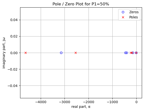

The code below generates a table that lists the values of the pole and zero locations.

table_header = ['Zeros, Hz', 'Poles, Hz']
num_table_rows = max(len(sys_zeros),len(sys_poles))
table_row = []

for i in range(num_table_rows):
    if i < len(sys_zeros):
        z = '{:.2f}'.format(sys_zeros[i]/(2*np.pi))
    else:
        z = ''
    if i < len(sys_poles):
        p = '{:.2f}'.format(sys_poles[i]/(2*np.pi))
    else:
        p = ''
    table_row.append([z,p])

print(tabulate(table_row, headers=table_header,colalign = ('left','left'),tablefmt="simple"))

Zeros, Hz    Poles, Hz
-----------  -----------
-3142.62     -4629.79
-458.92      -2545.69
-408.09      -231.62
-151.29      -180.17
-6.59        -6.6

39.3.3.2 Pole/Zero Locus Plot versus P1 value

There are 5 zeros and poles in the voltage transfer function. Solutions for the values of the poles and zeros as a function of \(P_1\)’s rotational position are saved to an array.

p1_value = 100e3
num_roots = []
denom_roots = []
for i in np.linspace(1,99,20)/100:
    element_values[Rp1a2] = p1_value - i*p1_value
    element_values[Rp1b2] = i*p1_value
    
    NE = NE_sym.subs(element_values)
    U = solve(NE,X)
    H = U[v2]/U[v1]
    num, denom = fraction(H) #returns numerator and denominator

    # convert symbolic to NumPy polynomial
    a = np.array(Poly(num, s).all_coeffs(), dtype=float)
    b = np.array(Poly(denom, s).all_coeffs(), dtype=float)    
    sys_tf = signal.TransferFunction(a,b)
    
    num_roots.append(np.roots(sys_tf.num))
    denom_roots.append(np.roots(sys_tf.den))

# put the zeros into an array
z0_locus = np.zeros(len(np.array(num_roots)))
z1_locus = np.zeros(len(np.array(num_roots)))
z2_locus = np.zeros(len(np.array(num_roots)))
z3_locus = np.zeros(len(np.array(num_roots)))
z4_locus = np.zeros(len(np.array(num_roots)))

for i in range(len(np.array(num_roots))):
    z0_locus[i] = -np.array(num_roots)[i][0]    
    z1_locus[i] = -np.array(num_roots)[i][1]        
    z2_locus[i] = -np.array(num_roots)[i][2]    
    z3_locus[i] = -np.array(num_roots)[i][3]  
    z4_locus[i] = -np.array(num_roots)[i][4]    
    
# put the poles into an array
p0_locus = np.zeros(len(np.array(denom_roots)))
p1_locus = np.zeros(len(np.array(denom_roots)))
p2_locus = np.zeros(len(np.array(denom_roots)))
p3_locus = np.zeros(len(np.array(denom_roots)))
p4_locus = np.zeros(len(np.array(denom_roots)))

for i in range(len(np.array(denom_roots))):
    p0_locus[i] = -np.array(denom_roots)[i][0]    
    p1_locus[i] = -np.array(denom_roots)[i][1]       
    p2_locus[i] = -np.array(denom_roots)[i][2]      
    p3_locus[i] = -np.array(denom_roots)[i][3]      
    p4_locus[i] = -np.array(denom_roots)[i][4]      

The range of values the zeros take on as a function of \(P_1\) is printed below.

print(f'z0 range as a function of P1: {z0_locus.min()/(2*np.pi)/1e3:.3f} to {z0_locus.max()/(2*np.pi)/1e3:.3f} kHz')
print(f'z1 range as a function of P1: {z1_locus.min()/(2*np.pi)/1e3:.3f} to {z1_locus.max()/(2*np.pi)/1e3:.3f} kHz')
print(f'z2 range as a function of P1: {z2_locus.min()/(2*np.pi)/1e3:.3f} to {z2_locus.max()/(2*np.pi)/1e3:.3f} kHz')
print(f'z3 range as a function of P1: {z3_locus.min()/(2*np.pi)/1e3:.3f} to {z3_locus.max()/(2*np.pi)/1e3:.3f} kHz')
print(f'z4 range as a function of P1: {z4_locus.min()/(2*np.pi)/1e3:.3f} to {z4_locus.max()/(2*np.pi)/1e3:.3f} kHz')

z0 range as a function of P1: 3.143 to 3.143 kHz
z1 range as a function of P1: 0.459 to 0.459 kHz
z2 range as a function of P1: 0.408 to 0.408 kHz
z3 range as a function of P1: 0.151 to 0.151 kHz
z4 range as a function of P1: 0.007 to 0.007 kHz

As shown above, the zeros of the transfer function don’t change with \(P_1\).

The range of values the poles take on as a function of \(P_1\) is printed below.

print(f'p0 range as a function of P1: {p0_locus.min()/(2*np.pi)/1e3:.3f} to {p0_locus.max()/(2*np.pi)/1e3:.3f} kHz')
print(f'p1 range as a function of P1: {p1_locus.min()/(2*np.pi)/1e3:.3f} to {p1_locus.max()/(2*np.pi)/1e3:.3f} kHz')
print(f'p2 range as a function of P1: {p2_locus.min()/(2*np.pi)/1e3:.3f} to {p2_locus.max()/(2*np.pi)/1e3:.3f} kHz')
print(f'p3 range as a function of P1: {p3_locus.min()/(2*np.pi)/1e3:.3f} to {p3_locus.max()/(2*np.pi)/1e3:.3f} kHz')
print(f'p4 range as a function of P1: {p4_locus.min()/(2*np.pi)/1e3:.3f} to {p4_locus.max()/(2*np.pi)/1e3:.3f} kHz')

p0 range as a function of P1: 4.611 to 5.043 kHz
p1 range as a function of P1: 2.546 to 3.046 kHz
p2 range as a function of P1: 0.232 to 0.455 kHz
p3 range as a function of P1: 0.179 to 0.181 kHz
p4 range as a function of P1: 0.007 to 0.007 kHz

As shown above the poles of the transfer function vary with \(P_1\), and these are plotted below.

plt.plot(np.linspace(1,99,len(np.array(denom_roots))),p0_locus/(2*np.pi)/1e3,'x-', markerfacecolor='none',label='p_0')
plt.plot(np.linspace(1,99,len(np.array(denom_roots))),p1_locus/(2*np.pi)/1e3,'x-', markerfacecolor='none',label='p_1')
plt.plot(np.linspace(1,99,len(np.array(denom_roots))),p2_locus/(2*np.pi)/1e3,'x-', markerfacecolor='none',label='p_2')
plt.plot(np.linspace(1,99,len(np.array(denom_roots))),p3_locus/(2*np.pi)/1e3,'x-', markerfacecolor='none',label='p_3')

plt.ylim((0,6))
plt.legend(loc='upper left')
plt.title('Gain control pole frequency plot vs gain pot rotation %')
plt.xlabel('Gain rotation percentage')
plt.ylabel('pole and zero frequency, kHz')
plt.grid()

plt.show()

As shown in the plots above, the pole locations don’t change all that much as a function of \(P_1\) rotation.

39.3.3.3 Reactive Branch 3 Frequency Response

The plot below shows the magnitude and phase of voltage transfer function versus frequency at various positions of \(P_1\).

# setup
x_axis = np.logspace(1, 5, 2000, endpoint=False)*2*np.pi
color_list = ['tab:blue','tab:red','tab:green','tab:orange','k']
gain_setting = np.array([1,25,50,75,99])/100
p1_value = 100e3

# plot
fig, ax1 = plt.subplots()
ax1.set_ylabel('magnitude, dB')
ax1.set_xlabel('frequency, Hz')

# instantiate a second y-axes that shares the same x-axis
ax2 = ax1.twinx()
color = 'k'

ax2.set_ylabel('phase, deg',color=color)
ax2.tick_params(axis='y', labelcolor=color)

for i in range(len(gain_setting)):
    element_values[Rp1a2] = p1_value - gain_setting[i]*p1_value
    element_values[Rp1b2] = gain_setting[i]*p1_value
    
    #element_values[Rp1a2] = p1_value - gain_setting[i]*p1_value
    #element_values[Rp1b2] = gain_setting[i]*p1_value
    
    NE = NE_sym.subs(element_values)
    U = solve(NE,X)
    H = U[v2]/U[v1]
    num, denom = fraction(H) #returns numerator and denominator

    # convert symbolic to NumPy polynomial
    a = np.array(Poly(num, s).all_coeffs(), dtype=float)
    b = np.array(Poly(denom, s).all_coeffs(), dtype=float)
    #tf_num_coef_list.append(a)
    #tf_denom_coef_list.append(b)
    
    #x = np.logspace(1, 5, 2000, endpoint=False)*2*np.pi
    w, mag, phase = signal.bode((a, b), w=x_axis) # returns: rad/s, mag in dB, phase in deg
    #clean_path1_mag[i] = mag
    
    # plot the results.  
    ax1.semilogx(w/(2*np.pi), mag,'-',color=color_list[i],label='mag: {:.0f}%'.format(gain_setting[i]*100))    # magnitude plot
    ax2.semilogx(w/(2*np.pi), phase,':',color=color_list[i],label='phase: {:.0f}%'.format(gain_setting[i]*100))  # phase plot

# highlight the guitar audio band, 80 to 8kHz
plt.axvspan(80, 8e3, color='y', alpha=0.3) 

# position legends outside the graph
ax1.legend(bbox_to_anchor=(1.6,1)) # magnitude legend position: relative (horizontal position, vertical position) 
ax2.legend(bbox_to_anchor=(1.6,0.5)) # phase legend position:

#ax1.legend(loc='lower left')
#ax2.legend(loc='lower right')
ax1.grid()
plt.title('Magnitude and phase response')
#plt.savefig('plt_rb_3.png')
plt.show()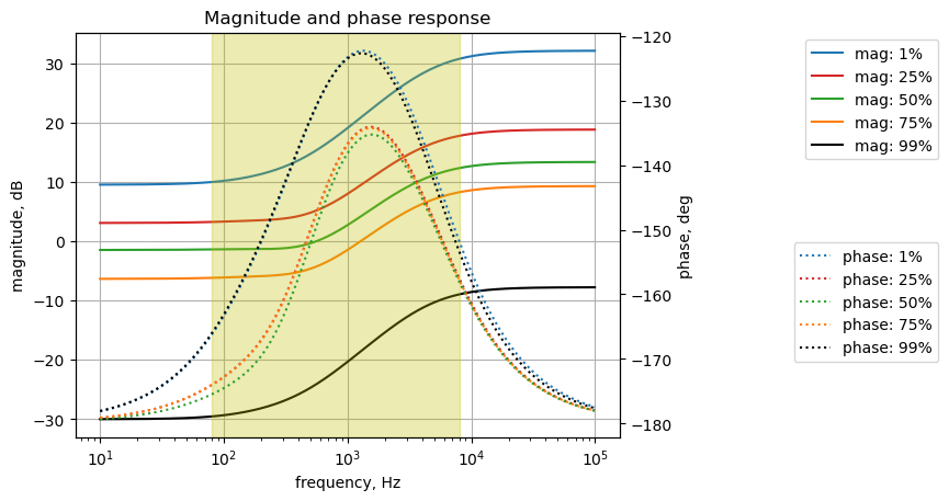

The magnitude and phase of voltage transfer function for reactive branch 3 shows about a 20 dB increase in gain over the guitar frequency band.

Keep in mind that \(C_{13}\) and \(R_{20}\) put a pole into the voltage transfer function at about 500 Hz, which reduces the frequency emphasis plotted above. This can be easily seen if \(C_{13}\) is included in the netlist and the analysis above is re-run. Poles and zeros with C13 as shown below, notice the addition of a pole at 495 Hz.

Zeros, Hz    Poles, Hz
-----------  -----------
-3142.62     -4629.79
-458.92      -2545.69
-408.09      -495.13
-151.29      -231.62
-6.59        -180.17
             -6.6

The plot of transfer function with \(C_{13}\) included in the analysis is:

Frequency response of reactive branch 3 with C13 included in the analysis.

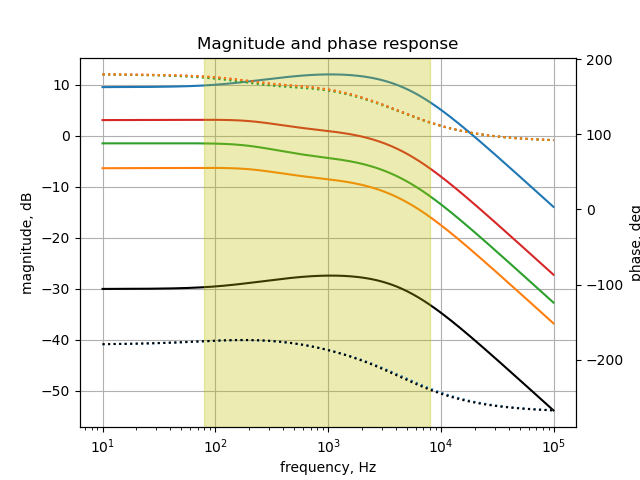
Notice that zero at 500 Hz now dominates the shape of the transfer function, which is now somewhat flat over the guitar band and a low pass filter with a cutoff starting around 3 kHz.

39.3.4 Reactive Branch 3a

The schematic shown below is a sub-circuit of reactive branch 3 from \(V_1\) to \(P_1\) (in the schematic below, the reference designator for \(P_1\) is \(R_{p1ab2}\) since \(P_1\) is modeled as two resistors.). In Figure 39.4, the nodes have been renumbered and \(P_1\) has been replaced by a fixed value resistor of 100 k\(\Omega\).

The branch from node 1 to node 3 is composed of components \(R_5\) and \(C_4\), and these have a resonant frequency of about 450 Hz. \(R_5\) and \(C_4\) are in parallel with each other and in series with the signal path and this arrangement forms a zero in the voltage transfer function. The components \(R_9\) and \(C_6\) are in series with each other and have a resonant frequency of about 400 Hz and present a shunt to the signal path, which produces a second zero in the voltage transfer function. By inspection we can see the gain is \((R_8||P_1)/(R_5+R_8||P_1)\) at \(\omega=0\) since the capacitors are open circuits at DC. At high frequency the gain is 1 since \(C_4\) looks like a short at high frequency.

Figure 39.4: Schematic of reactive branch 3a.

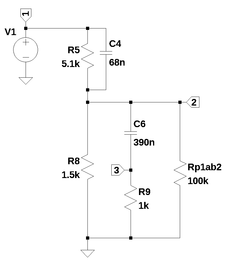
The netlist below was obtained from the LTSpice schematic.

reactive_branch_3_4_a_net_list = '''
* Reactive_branch_3&4_a.asc
R5 1 2 5.1e3
R8 2 0 1.5e3
C4 1 2 68e-9
C6 2 3 390e-9
R9 3 0 1e3
Rp1ab2 2 0 100e3
V1 1 0 1
'''

The MNA matrices are generated by calling SymMNA.smna.

report, network_df, i_unk_df, A, X, Z = SymMNA.smna(reactive_branch_3_4_a_net_list)

The network equations are built from the MNA matrices.

# Put matrices into SymPy 
X = Matrix(X)
Z = Matrix(Z)

NE_sym = Eq(A*X,Z)

# display the equations
temp = ''
for i in range(shape(NE_sym.lhs)[0]):
    temp += '${:s} = {:s}$<br>'.format(latex(NE_sym.rhs[i]),latex(NE_sym.lhs[i]))
Markdown(temp)

\(0 = I_{V1} + v_{1} \left(C_{4} s + \frac{1}{R_{5}}\right) + v_{2} \left(- C_{4} s - \frac{1}{R_{5}}\right)\)
\(0 = - C_{6} s v_{3} + v_{1} \left(- C_{4} s - \frac{1}{R_{5}}\right) + v_{2} \left(C_{4} s + C_{6} s + \frac{1}{Rp1ab2} + \frac{1}{R_{8}} + \frac{1}{R_{5}}\right)\)
\(0 = - C_{6} s v_{2} + v_{3} \left(C_{6} s + \frac{1}{R_{9}}\right)\)
\(V_{1} = v_{1}\)

The free symbols are turned into SymPy symbols and the element values are loaded into a dictionary.

var(str(NE_sym.free_symbols).replace('{','').replace('}',''))
element_values = SymMNA.get_part_values(network_df)

39.3.4.1 Symbolic solution

The network equations can be solved symbolically and are displayed below.

U_sym = solve(NE_sym,X)

temp = ''
for i in U_sym.keys():
    temp += '${:s} = {:s}$<br>'.format(latex(i),latex(U_sym[i]))

Markdown(temp)

\(v_{1} = V_{1}\)
\(v_{2} = \frac{C_{4} C_{6} R_{5} R_{8} R_{9} Rp1ab2 V_{1} s^{2} + C_{4} R_{5} R_{8} Rp1ab2 V_{1} s + C_{6} R_{8} R_{9} Rp1ab2 V_{1} s + R_{8} Rp1ab2 V_{1}}{C_{4} C_{6} R_{5} R_{8} R_{9} Rp1ab2 s^{2} + C_{4} R_{5} R_{8} Rp1ab2 s + C_{6} R_{5} R_{8} R_{9} s + C_{6} R_{5} R_{8} Rp1ab2 s + C_{6} R_{5} R_{9} Rp1ab2 s + C_{6} R_{8} R_{9} Rp1ab2 s + R_{5} R_{8} + R_{5} Rp1ab2 + R_{8} Rp1ab2}\)
\(v_{3} = \frac{C_{4} C_{6} R_{5} R_{8} R_{9} Rp1ab2 V_{1} s^{2} + C_{6} R_{8} R_{9} Rp1ab2 V_{1} s}{C_{4} C_{6} R_{5} R_{8} R_{9} Rp1ab2 s^{2} + C_{4} R_{5} R_{8} Rp1ab2 s + C_{6} R_{5} R_{8} R_{9} s + C_{6} R_{5} R_{8} Rp1ab2 s + C_{6} R_{5} R_{9} Rp1ab2 s + C_{6} R_{8} R_{9} Rp1ab2 s + R_{5} R_{8} + R_{5} Rp1ab2 + R_{8} Rp1ab2}\)
\(I_{V1} = \frac{- C_{4} C_{6} R_{5} R_{8} R_{9} V_{1} s^{2} - C_{4} C_{6} R_{5} R_{8} Rp1ab2 V_{1} s^{2} - C_{4} C_{6} R_{5} R_{9} Rp1ab2 V_{1} s^{2} - C_{4} R_{5} R_{8} V_{1} s - C_{4} R_{5} Rp1ab2 V_{1} s - C_{6} R_{8} R_{9} V_{1} s - C_{6} R_{8} Rp1ab2 V_{1} s - C_{6} R_{9} Rp1ab2 V_{1} s - R_{8} V_{1} - Rp1ab2 V_{1}}{C_{4} C_{6} R_{5} R_{8} R_{9} Rp1ab2 s^{2} + C_{4} R_{5} R_{8} Rp1ab2 s + C_{6} R_{5} R_{8} R_{9} s + C_{6} R_{5} R_{8} Rp1ab2 s + C_{6} R_{5} R_{9} Rp1ab2 s + C_{6} R_{8} R_{9} Rp1ab2 s + R_{5} R_{8} + R_{5} Rp1ab2 + R_{8} Rp1ab2}\)

SymPy can solve and display the node voltage equations.

U_sym = solve(NE_sym,X)

temp = ''
for i in U_sym.keys():
    temp += '${:s} = {:s}$<br>'.format(latex(i),latex(U_sym[i]))

Markdown(temp)

\(v_{1} = V_{1}\)
\(v_{2} = \frac{C_{4} C_{6} R_{5} R_{8} R_{9} Rp1ab2 V_{1} s^{2} + C_{4} R_{5} R_{8} Rp1ab2 V_{1} s + C_{6} R_{8} R_{9} Rp1ab2 V_{1} s + R_{8} Rp1ab2 V_{1}}{C_{4} C_{6} R_{5} R_{8} R_{9} Rp1ab2 s^{2} + C_{4} R_{5} R_{8} Rp1ab2 s + C_{6} R_{5} R_{8} R_{9} s + C_{6} R_{5} R_{8} Rp1ab2 s + C_{6} R_{5} R_{9} Rp1ab2 s + C_{6} R_{8} R_{9} Rp1ab2 s + R_{5} R_{8} + R_{5} Rp1ab2 + R_{8} Rp1ab2}\)
\(v_{3} = \frac{C_{4} C_{6} R_{5} R_{8} R_{9} Rp1ab2 V_{1} s^{2} + C_{6} R_{8} R_{9} Rp1ab2 V_{1} s}{C_{4} C_{6} R_{5} R_{8} R_{9} Rp1ab2 s^{2} + C_{4} R_{5} R_{8} Rp1ab2 s + C_{6} R_{5} R_{8} R_{9} s + C_{6} R_{5} R_{8} Rp1ab2 s + C_{6} R_{5} R_{9} Rp1ab2 s + C_{6} R_{8} R_{9} Rp1ab2 s + R_{5} R_{8} + R_{5} Rp1ab2 + R_{8} Rp1ab2}\)
\(I_{V1} = \frac{- C_{4} C_{6} R_{5} R_{8} R_{9} V_{1} s^{2} - C_{4} C_{6} R_{5} R_{8} Rp1ab2 V_{1} s^{2} - C_{4} C_{6} R_{5} R_{9} Rp1ab2 V_{1} s^{2} - C_{4} R_{5} R_{8} V_{1} s - C_{4} R_{5} Rp1ab2 V_{1} s - C_{6} R_{8} R_{9} V_{1} s - C_{6} R_{8} Rp1ab2 V_{1} s - C_{6} R_{9} Rp1ab2 V_{1} s - R_{8} V_{1} - Rp1ab2 V_{1}}{C_{4} C_{6} R_{5} R_{8} R_{9} Rp1ab2 s^{2} + C_{4} R_{5} R_{8} Rp1ab2 s + C_{6} R_{5} R_{8} R_{9} s + C_{6} R_{5} R_{8} Rp1ab2 s + C_{6} R_{5} R_{9} Rp1ab2 s + C_{6} R_{8} R_{9} Rp1ab2 s + R_{5} R_{8} + R_{5} Rp1ab2 + R_{8} Rp1ab2}\)

The network transfer function, \(H(s)=\frac {v_2(s)}{v_1(s)}\) is:

H_sym = (U_sym[v2]/U_sym[v1]).cancel()
Markdown('$H(s)={:s}$'.format(latex(H_sym)))

\(H(s)=\frac{C_{4} C_{6} R_{5} R_{8} R_{9} Rp1ab2 s^{2} + C_{4} R_{5} R_{8} Rp1ab2 s + C_{6} R_{8} R_{9} Rp1ab2 s + R_{8} Rp1ab2}{C_{4} C_{6} R_{5} R_{8} R_{9} Rp1ab2 s^{2} + C_{4} R_{5} R_{8} Rp1ab2 s + C_{6} R_{5} R_{8} R_{9} s + C_{6} R_{5} R_{8} Rp1ab2 s + C_{6} R_{5} R_{9} Rp1ab2 s + C_{6} R_{8} R_{9} Rp1ab2 s + R_{5} R_{8} + R_{5} Rp1ab2 + R_{8} Rp1ab2}\)

We can look at the numerator and denominator polynomials of the transfer function.

H_sym_num, H_sym_denom = fraction(H_sym,s) #returns numerator and denominator

39.3.4.2 Numerator Polynomial

The numerator polynomial is:

Markdown('$N(s)={:s}$'.format(latex(H_sym_num)))

\(N(s)=C_{4} C_{6} R_{5} R_{8} R_{9} Rp1ab2 s^{2} + C_{4} R_{5} R_{8} Rp1ab2 s + C_{6} R_{8} R_{9} Rp1ab2 s + R_{8} Rp1ab2\)

The coefficients of each Laplace term can be equated to the variables \(b_2\), \(b_1\) and \(b_0\) in the expression:

\(b_2s^{2}+b_1s+b_0\)

where \(b_2\), \(b_1\) and \(b_0\) are:

b2 = H_sym_num.coeff(s**2)
b1 = H_sym_num.coeff(s**1)
b0 = (H_sym_num - b1*s*1 - b2*s**2).expand()

Markdown('<p>$b_2={:s}$</p><p>$b_1={:s}$\
    </p><p>$b_0={:s}$</p>'.format(latex(b2),latex(b1),latex(b0)))

\(b_2=C_{4} C_{6} R_{5} R_{8} R_{9} Rp1ab2\)

\(b_1=C_{4} R_{5} R_{8} Rp1ab2 + C_{6} R_{8} R_{9} Rp1ab2\)

\(b_0=R_{8} Rp1ab2\)

The roots of the numerator polynomial can easily be found with SymPy. This filter has two transmission zeros, which can be found using the solve function on the numerator polynomial.

num_root_sym = solve(H_sym_num,s)

Markdown('There are {:d} zeros, which are:\
    <p>$z_0={:s}$</p><p>$z_1={:s}$</p>'.format(len(num_root_sym),latex(num_root_sym[0]),latex(num_root_sym[1])))

There are 2 zeros, which are:

\(z_0=- \frac{1}{C_{4} R_{5}}\)

\(z_1=- \frac{1}{C_{6} R_{9}}\)

39.3.4.3 Denominator Polynomial

The denominator polynomial of the transfer function is called the characteristic polynomial. The roots of the denominator, also called poles of the system, determine the system’s stability. If any of these roots have a positive real part, the system is unstable, meaning its output will grow unbounded. The roots also influence how the system responds to changes in input (the transient response). They affect things like how quickly the system settles to a new state, whether it oscillates, and the damping of those oscillations. Each root of the characteristic polynomial corresponds to a natural mode of the system.

The denominator polynomial is:

Markdown('$D(s)={:s}$'.format(latex(H_sym_denom)))

\(D(s)=C_{4} C_{6} R_{5} R_{8} R_{9} Rp1ab2 s^{2} + C_{4} R_{5} R_{8} Rp1ab2 s + C_{6} R_{5} R_{8} R_{9} s + C_{6} R_{5} R_{8} Rp1ab2 s + C_{6} R_{5} R_{9} Rp1ab2 s + C_{6} R_{8} R_{9} Rp1ab2 s + R_{5} R_{8} + R_{5} Rp1ab2 + R_{8} Rp1ab2\)

The coefficients of each Laplace term can be equated to the variables \(a_2\), \(a_1\) and \(a_0\) in the expression:

\(a_2s^2+a_1s+a_0\)

where \(a_2\), \(a_1\) and \(a_0\) are:

\(a_2=C_{4} C_{6} R_{5} R_{8} R_{9} Rp1ab2\)

\(a_1=C_{4} R_{5} R_{8} Rp1ab2 + C_{6} R_{5} R_{8} R_{9} + C_{6} R_{5} R_{8} Rp1ab2 + C_{6} R_{5} R_{9} Rp1ab2 + C_{6} R_{8} R_{9} Rp1ab2\)

\(a_0=R_{5} R_{8} + R_{5} Rp1ab2 + R_{8} Rp1ab2\)

The roots of the denominator polynomial, which are the poles of the transder fuction, can be found with SymPy.

denom_root_sym = solve(H_sym_denom,s)

Markdown('There are {:d} poles, which are:\
    <p>$p_0={:s}$</p><p>$p_1={:s}$</p>'.format(len(denom_root_sym),latex(denom_root_sym[0]),latex(denom_root_sym[1])))

There are 2 poles, which are:

\(p_0=\frac{- C_{4} R_{5} R_{8} Rp1ab2 - C_{6} R_{5} R_{8} R_{9} - C_{6} R_{5} R_{8} Rp1ab2 - C_{6} R_{5} R_{9} Rp1ab2 - C_{6} R_{8} R_{9} Rp1ab2 - \sqrt{C_{4}^{2} R_{5}^{2} R_{8}^{2} Rp1ab2^{2} - 2 C_{4} C_{6} R_{5}^{2} R_{8}^{2} R_{9} Rp1ab2 + 2 C_{4} C_{6} R_{5}^{2} R_{8}^{2} Rp1ab2^{2} - 2 C_{4} C_{6} R_{5}^{2} R_{8} R_{9} Rp1ab2^{2} - 2 C_{4} C_{6} R_{5} R_{8}^{2} R_{9} Rp1ab2^{2} + C_{6}^{2} R_{5}^{2} R_{8}^{2} R_{9}^{2} + 2 C_{6}^{2} R_{5}^{2} R_{8}^{2} R_{9} Rp1ab2 + C_{6}^{2} R_{5}^{2} R_{8}^{2} Rp1ab2^{2} + 2 C_{6}^{2} R_{5}^{2} R_{8} R_{9}^{2} Rp1ab2 + 2 C_{6}^{2} R_{5}^{2} R_{8} R_{9} Rp1ab2^{2} + C_{6}^{2} R_{5}^{2} R_{9}^{2} Rp1ab2^{2} + 2 C_{6}^{2} R_{5} R_{8}^{2} R_{9}^{2} Rp1ab2 + 2 C_{6}^{2} R_{5} R_{8}^{2} R_{9} Rp1ab2^{2} + 2 C_{6}^{2} R_{5} R_{8} R_{9}^{2} Rp1ab2^{2} + C_{6}^{2} R_{8}^{2} R_{9}^{2} Rp1ab2^{2}}}{2 C_{4} C_{6} R_{5} R_{8} R_{9} Rp1ab2}\)

\(p_1=\frac{- C_{4} R_{5} R_{8} Rp1ab2 - C_{6} R_{5} R_{8} R_{9} - C_{6} R_{5} R_{8} Rp1ab2 - C_{6} R_{5} R_{9} Rp1ab2 - C_{6} R_{8} R_{9} Rp1ab2 + \sqrt{C_{4}^{2} R_{5}^{2} R_{8}^{2} Rp1ab2^{2} - 2 C_{4} C_{6} R_{5}^{2} R_{8}^{2} R_{9} Rp1ab2 + 2 C_{4} C_{6} R_{5}^{2} R_{8}^{2} Rp1ab2^{2} - 2 C_{4} C_{6} R_{5}^{2} R_{8} R_{9} Rp1ab2^{2} - 2 C_{4} C_{6} R_{5} R_{8}^{2} R_{9} Rp1ab2^{2} + C_{6}^{2} R_{5}^{2} R_{8}^{2} R_{9}^{2} + 2 C_{6}^{2} R_{5}^{2} R_{8}^{2} R_{9} Rp1ab2 + C_{6}^{2} R_{5}^{2} R_{8}^{2} Rp1ab2^{2} + 2 C_{6}^{2} R_{5}^{2} R_{8} R_{9}^{2} Rp1ab2 + 2 C_{6}^{2} R_{5}^{2} R_{8} R_{9} Rp1ab2^{2} + C_{6}^{2} R_{5}^{2} R_{9}^{2} Rp1ab2^{2} + 2 C_{6}^{2} R_{5} R_{8}^{2} R_{9}^{2} Rp1ab2 + 2 C_{6}^{2} R_{5} R_{8}^{2} R_{9} Rp1ab2^{2} + 2 C_{6}^{2} R_{5} R_{8} R_{9}^{2} Rp1ab2^{2} + C_{6}^{2} R_{8}^{2} R_{9}^{2} Rp1ab2^{2}}}{2 C_{4} C_{6} R_{5} R_{8} R_{9} Rp1ab2}\)

39.3.5 Analysis Using the Extra Element Theorem

The coefficients of the numerator and denominator polynomials for the transfer function of the circuit shown in Figure 39.4 can be determined by using the N Extra Element Theorem of Middlebrook, Vorperian, and Lindal (1998). Since there are only two reactive components in the circuit, this can be performed by inspection. See the example starting on slide 85 of Basso (2016). The following code cells walk through the steps.

The denominator polynomial coefficients \(c_2\) and \(c_1\) in the expression:

\(c_2s^2+c_1s+1\)

can be found by the following steps. First find the time constants \(\tau_1\) and \(\tau_2\) while \(V_1=0\). To find \(\tau_1\), look at Figure 39.4 with \(V_1=0\) and \(C_6\) replaced by its impedance at \(\omega=0\), which is an open circuit. The resistance seen by \(C_4\) is the parallel combination of \(R_5\), \(R_8\) and \(R_{p1ab2}\) which is equal to \(\frac {1} {\frac {1}{R_5}+\frac {1}{R_8}+\frac {1}{R_{p1ab2}} }\). We can create a new symbol \(Rp\) to represent the parallel combination of \(R_5\), \(R_8\) and \(R_{p1ab2}\).

Rp = symbols('Rp')

tau_1 = C4*Rp
Markdown('The time constant $\\tau_1 = {:s}$.'.format(latex(tau_1)))

The time constant \(\tau_1 = C_{4} Rp\).

To find \(\tau_2\), replace \(C_4\) its impedance at \(\omega=0\), which is an open circuit. The resistance seen by \(C_6\) is \(R_9\) plus the parallel combination of \(R_5\), \(R_8\) and \(R_{p1ab2}\) which is equal to \(R_9 + \frac {1} {\frac {1}{R_5}+\frac {1}{R_8}+\frac {1}{R_{p1ab2}} }\).

tau_2 = C6*(Rp+R9)
Markdown('The time constant $\\tau_2 = {:s}$.'.format(latex(tau_2)))

The time constant \(\tau_2 = C_{6} \left(R_{9} + Rp\right)\).

c_1 = tau_1+tau_2
Markdown('The denominator polynomial coefficient, $c_1 = \\tau_1+\\tau_2 = {:s}$.'.format(latex(c_1)))

The denominator polynomial coefficient, \(c_1 = \tau_1+\tau_2 = C_{4} Rp + C_{6} \left(R_{9} + Rp\right)\).

To find \(c_2\), place C1 in its high-frequency and look into C2, \(V_1\) is still zero, this is \(\tau_1^2\) and \(a_2 = \tau_1 \tau_1^2\).

# tau_1^2
tau_1_2 = (C6*R9)
Markdown('$\\tau_1^2 = {:s}$'.format(latex(tau_1_2)))

\(\tau_1^2 = C_{6} R_{9}\)

The second coeeficient is equal to \(\tau_1 \tau_1^2\).

c_2 = tau_1*tau_1_2
Markdown('$c_2 = {:s}$'.format(latex(c_2)))

\(c_2 = C_{4} C_{6} R_{9} Rp\)

Markdown('The denominator polynomial = ${:s}$'.format(latex(c_2*s**2+c_1*s+1)))

The denominator polynomial = \(C_{4} C_{6} R_{9} Rp s^{2} + s \left(C_{4} Rp + C_{6} \left(R_{9} + Rp\right)\right) + 1\)

To find if \(C_4\) and \(C_6\) cause zeros in the transfer function, the following procedure is used:

• Place \(C_4\) in its high-frequency state while \(C_6\) is in its low frequency state, check if the stimulus can propagate through the circuit to form a response on the output.
• The place \(C_6\) in its high-frequency state while \(C_4\) is in its low frequency state, check if the stimulus can propagate through the circuit to form a response on the output.

In both cases the stimulus can propagate through the circuit to form a response on the output.

To find the locations of the zeros, you have to find the impedance condition in the circuit where, for a certain stimulus frequency, you null the response. Either a series impedance becomes an infinite value or a shunt branch is zero. This happens for:

t1 = C6*R9
t2 = C4*R5
Markdown('$t_1 = C_6R_9$ and $t_2 = C_4R_5$')

\(t_1 = C_6R_9\) and \(t_2 = C_4R_5\)

Markdown('We can write the numerator polynomial in factored form: ${:s}$'.format(latex((s+1/t1)*(s+1/t2))))

We can write the numerator polynomial in factored form: \(\left(s + \frac{1}{C_{4} R_{5}}\right) \left(s + \frac{1}{C_{6} R_{9}}\right)\)

The DC gain of the transfer function, \(H_0\) can be found by letting \(\omega=0\) and is:

\(H_0=\frac{R_8||P_1}{R_5+R_8||P_1}\)

Now we can write the transfer function:

H_0 = symbols('H_0')
Markdown('$H(s)={:s}$'.format(latex(H_0*(s+1/t1)*(s+1/t2)/(c_2*s**2+c_1*s+1))))

\(H(s)=\frac{H_{0} \left(s + \frac{1}{C_{4} R_{5}}\right) \left(s + \frac{1}{C_{6} R_{9}}\right)}{C_{4} C_{6} R_{9} Rp s^{2} + s \left(C_{4} Rp + C_{6} \left(R_{9} + Rp\right)\right) + 1}\)

The expression obtained for \(H(s)\) above can be checked by substituting element values and comparing to the MNA results above.

Substituting \(R_{p1ab2}\) for \(P_1\), the expression for \(H_0\) is:

H_0 = (1/(1/R8+1/Rp1ab2))/(R5+1/(1/R8+1/Rp1ab2))
Markdown('$H_0(s)={:s}$'.format(latex(H_0)))

\(H_0(s)=\frac{1}{\left(R_{5} + \frac{1}{\frac{1}{Rp1ab2} + \frac{1}{R_{8}}}\right) \left(\frac{1}{Rp1ab2} + \frac{1}{R_{8}}\right)}\)

Putting all the sysmbols together, we get:

Markdown('$H(s)={:s}$'.format(latex(H_0*(s+1/t1)*(s+1/t2)/(c_2*s**2+c_1*s+1))))

\(H(s)=\frac{\left(s + \frac{1}{C_{4} R_{5}}\right) \left(s + \frac{1}{C_{6} R_{9}}\right)}{\left(R_{5} + \frac{1}{\frac{1}{Rp1ab2} + \frac{1}{R_{8}}}\right) \left(\frac{1}{Rp1ab2} + \frac{1}{R_{8}}\right) \left(C_{4} C_{6} R_{9} Rp s^{2} + s \left(C_{4} Rp + C_{6} \left(R_{9} + Rp\right)\right) + 1\right)}\)

Making the substitution for \(R_P\) we get:

H = (H_0*(s+1/t1)*(s+1/t2)/(c_2*s**2+c_1*s+1)).subs({Rp:1/(1/R5+1/R8+1/Rp1ab2)})
Markdown('$H(s)={:s}$'.format(latex(H)))

\(H(s)=\frac{\left(s + \frac{1}{C_{4} R_{5}}\right) \left(s + \frac{1}{C_{6} R_{9}}\right)}{\left(R_{5} + \frac{1}{\frac{1}{Rp1ab2} + \frac{1}{R_{8}}}\right) \left(\frac{1}{Rp1ab2} + \frac{1}{R_{8}}\right) \left(\frac{C_{4} C_{6} R_{9} s^{2}}{\frac{1}{Rp1ab2} + \frac{1}{R_{8}} + \frac{1}{R_{5}}} + s \left(\frac{C_{4}}{\frac{1}{Rp1ab2} + \frac{1}{R_{8}} + \frac{1}{R_{5}}} + C_{6} \left(R_{9} + \frac{1}{\frac{1}{Rp1ab2} + \frac{1}{R_{8}} + \frac{1}{R_{5}}}\right)\right) + 1\right)}\)

Putting in the element values we get:

H = H.subs(element_values)
Markdown('$H(s)={:s}$'.format(latex(H)))

\(H(s)=\frac{0.224668613794653 \left(s + 2564.10256410256\right) \left(s + 2883.50634371396\right)}{3.03868793529544 \cdot 10^{-8} s^{2} + 0.00091478094810155 s + 1}\)

Now we can extract the numerator and demoninator and compare to the MNA results.

H1_num, H1_denom = fraction(H)

The numerator obtained with the EET is:

H1_num.expand()/H1_num.expand().coeff(s**2)

\(\displaystyle 1.0 s^{2} + 5447.60890781652 s + 7393606.00952296\)

Which exactly matches the numberator obtained from MNA.

H_sym_num.subs(element_values)/H_sym_num.subs(element_values).coeff(s**2)

\(\displaystyle 1.0 s^{2} + 5447.60890781652 s + 7393606.00952297\)

Looking at the demominators, the demininator obtanained from the EET is :

H1_denom/H1_denom.coeff(s**2)

\(\displaystyle 1.0 s^{2} + 30104.4716529146 s + 32908940.3483867\)

Which exactly matches the demoninator obtained from MNA.

H_sym_denom.subs(element_values)/H_sym_denom.subs(element_values).coeff(s**2)

\(\displaystyle 1.0 s^{2} + 30104.4716529146 s + 32908940.3483867\)

This varifies that the EET solution is valid. If the circuit is a 2nd order circuit, this analysis approach can be useful.

39.3.5.1 Numerical Solution

If numerical values are substituted for the reference designators in the symbolic equations, the following numerical equations can be obtained.

equ_N = NE_sym.subs(element_values)

temp = ''
for i in range(shape(equ_N.lhs)[0]):
    temp += '<p>${:s} = {:s}$</p>'.format(latex(equ_N.rhs[i]),
        latex(round_expr(equ_N.lhs[i],8)))

Markdown(temp)

\(0 = I_{V1} + v_{1} \cdot \left(7.0 \cdot 10^{-8} s + 0.00019608\right) + v_{2} \left(- 7.0 \cdot 10^{-8} s - 0.00019608\right)\)

\(0 = - 3.9 \cdot 10^{-7} s v_{3} + v_{1} \left(- 7.0 \cdot 10^{-8} s - 0.00019608\right) + v_{2} \cdot \left(4.6 \cdot 10^{-7} s + 0.00087275\right)\)

\(0 = - 3.9 \cdot 10^{-7} s v_{2} + v_{3} \cdot \left(3.9 \cdot 10^{-7} s + 0.001\right)\)

\(1.0 = v_{1}\)

SymPy can solve for unknown node voltages and the unknown currents from the independent voltage source, \(V_1\), and the Op Amp’s output terminal. The unknown currents, \(I_{V1}\) and \(I_{O1}\), are not displayed. The node voltages are:

U = solve(equ_N,X)

temp = ''
for i in U.keys():
    if str(i)[0] == 'v': # only display the node voltages
        temp += '<p>${:s} = {:s}$</p>'.format(latex(i),latex(U[i]))

Markdown(temp)

\(v_{1} = 1.0\)

\(v_{2} = \frac{2652000000000.0 s^{2} + 1.44470588235294 \cdot 10^{16} s + 1.96078431372549 \cdot 10^{19}}{2652000000000.0 s^{2} + 7.98370588235294 \cdot 10^{16} s + 8.72745098039216 \cdot 10^{19}}\)

\(v_{3} = \frac{2652000000000.0 s^{2} + 7.64705882352941 \cdot 10^{15} s}{2652000000000.0 s^{2} + 7.98370588235294 \cdot 10^{16} s + 8.72745098039216 \cdot 10^{19}}\)

H = (U[v2]/U[v1]).cancel()
Markdown('The transfer function is: $H(s)={:s}$'.format(latex(H)))

The transfer function is: \(H(s)=\frac{2652000000000.0 s^{2} + 1.44470588235294 \cdot 10^{16} s + 1.96078431372549 \cdot 10^{19}}{2652000000000.0 s^{2} + 7.98370588235294 \cdot 10^{16} s + 8.72745098039216 \cdot 10^{19}}\)

The SciPy function, TransferFunction, is used to represent the system as the continuous-time transfer function. The code below extracts the numerator and denominator polynomials from the voltage transfer function. Then coefficients of the terms are used to build a SciPy transfer function object.

H_num, H_denom = fraction(H) #returns numerator and denominator

# convert symbolic to NumPy polynomial
a = np.array(Poly(H_num, s).all_coeffs(), dtype=float)
b = np.array(Poly(H_denom, s).all_coeffs(), dtype=float)

sys_tf = signal.TransferFunction(a,b)

sys_zeros = np.roots(sys_tf.num)
sys_poles = np.roots(sys_tf.den)

The poles and zeros of the transfer function are plotted on the complex frequency plane with the following code:

plt.plot(np.real(sys_zeros/(2*np.pi)), np.imag(sys_zeros/(2*np.pi)), 'ob', markerfacecolor='none')
plt.plot(np.real(sys_poles/(2*np.pi)), np.imag(sys_poles/(2*np.pi)), 'xr')
plt.legend(['Zeros', 'Poles'], loc=0)
plt.title('Pole / Zero Plot')
plt.xlabel('real part, \u03B1')
plt.ylabel('imaginary part, j\u03C9')
plt.grid()
plt.show()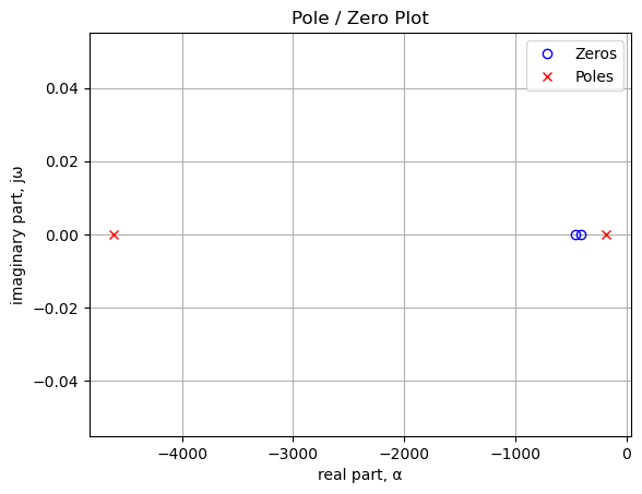

The code below generates a table that lists the values of the pole and zero locations.

table_header = ['Zeros, Hz', 'Poles, Hz']
num_table_rows = max(len(sys_zeros),len(sys_poles))
table_row = []

for i in range(num_table_rows):
    if i < len(sys_zeros):
        z = '{:.2f}'.format(sys_zeros[i]/(2*np.pi))
    else:
        z = ''
    if i < len(sys_poles):
        p = '{:.2f}'.format(sys_poles[i]/(2*np.pi))
    else:
        p = ''
    table_row.append([z,p])

print(tabulate(table_row, headers=table_header,colalign = ('left','left'),tablefmt="simple"))

Zeros, Hz    Poles, Hz
-----------  -----------
-458.92      -4610.47
-408.09      -180.8

39.3.5.2 Reactive Branch 3a Frequency Response

The frequency response for the circuit in Figure 39.4 is shown below.

# setup
x_axis = np.logspace(1, 5, 2000, endpoint=False)*2*np.pi
color_list = ['tab:blue','tab:red','tab:green','tab:orange','k']
#gain_setting = np.array([1,25,50,75,99])/100
#p1_value = 100e3

#tf_num_coef_list = []
#tf_denom_coef_list = []

#clean_path1_mag = np.zeros((len(gain_setting),len(x_axis)))

#color_list = ['tab:blue','tab:red','tab:green','tab:orange','k']

# plot
fig, ax1 = plt.subplots()
ax1.set_ylabel('magnitude, dB')
ax1.set_xlabel('frequency, Hz')

# instantiate a second y-axes that shares the same x-axis
ax2 = ax1.twinx()
color = 'k'

ax2.set_ylabel('phase, deg',color=color)
ax2.tick_params(axis='y', labelcolor=color)


NE = NE_sym.subs(element_values)
U = solve(NE,X)
H = U[v2]/U[v1]
num, denom = fraction(H) #returns numerator and denominator

# convert symbolic to NumPy polynomial
a = np.array(Poly(num, s).all_coeffs(), dtype=float)
b = np.array(Poly(denom, s).all_coeffs(), dtype=float)

#x = np.logspace(1, 5, 2000, endpoint=False)*2*np.pi
w, mag, phase = signal.bode((a, b), w=x_axis) # returns: rad/s, mag in dB, phase in deg
#clean_path1_mag[i] = mag

# plot the results
i=0
ax1.semilogx(w/(2*np.pi), mag,'-k',label='mag')    # magnitude plot
ax2.semilogx(w/(2*np.pi), phase,':k',label='phase')  # phase plot

# highlight the guitar audio band, 80 to 8kHz
plt.axvspan(80, 8e3, color='y', alpha=0.3) 

ax1.set_ylim((-20,5))

# position legends
ax1.legend(loc='upper left')
ax2.legend(loc='upper right')

ax1.grid()
plt.title('Magnitude and phase response')
plt.show()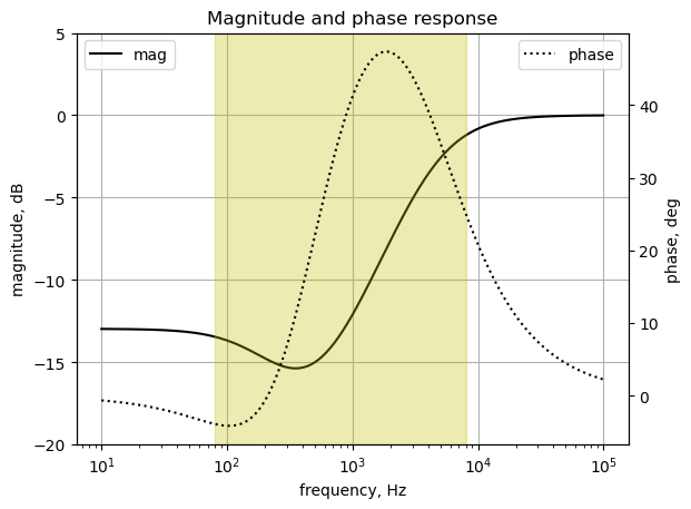

By examining the circuit in Figure 39.4, we can see that there is a DC path from node 1 to node 2. At \(\omega=0\), the capacitors act as open circuits and the circuit reduces to a voltage divider equal to \(\frac {R_8||P_1} {R_5+R_8||P_1}\) between nodes 1 and 2. At high frequencies, the capacitors act as short circuits and at high frequencies node 2 is shorted to node 1 by \(C_4\)

39.3.6 Reactive Branch 3b

The branch composed of components \(R_{15}\), \(C_{11}\) and \(R_{16}\) and the branch composed of components \(R_{17}\), \(R_{18}\) and \(C_{12}\), form an unusual summing network attached to node 10 in Figure 39.3. The signal from the diode path combines with the signal from clean path 2 through \(C_{11}\) at node 9.

The resistor \(R_{16}\) conducts this blended signal into the summing junction at node 10. The signal from clean path 2 travels through the branch composed of components \(R_{17}\), \(R_{18}\) and \(C_{12}\) to the summing junction at node 10. The branch from node 5 to node 10, consisting of components \(R_{17}\), \(R_{18}\) and \(C_{12}\), attaches to the summing junction at node 10 and combines the signal from clean path 2. These components have resonances that contribute to the poles and zeros of the transfer function.

The components \(R_{18}\) and \(C_{12}\) have a resonant frequency of about 500 Hz and since these are in series contribute to a pole to the transfer function at their resonant frequency. The components \(R_{18}+R_{17}\) and \(C_{12}\) have a resonant frequency of about 150 Hz and these contribute to a zero to the transfer function at their resonant frequency.

It’s not clear how the arrangement of these components attached to the summing junction were determined, perhaps this topology came to look like this by experimentation in the circuit prototyping and testing phase of the design.

When \(P_{1A}\) in Figure 37.17, is rotated fully clockwise the wiper is connected to the ground end and no signal propagates along the path. When \(P_{1A}\) is rotated fully counter clockwise, the wiper is connected to \(C_6\) and the clean signal can propagate along the path. Otherwise, \(P_{1A}\) acts as a voltage divider and the amplitude of the signal can be adjusted by the user.

The schematic in Figure 39.3 has been redrawn below, notice that the node numbers have changed. The capacitor values for \(C_{10}\) and \(C_9\) have been combined and 0.5 \(\mu\)F has been used for the value of \(C_{10}\) below.

Figure 39.5: Schematic of reactive branch 3b.

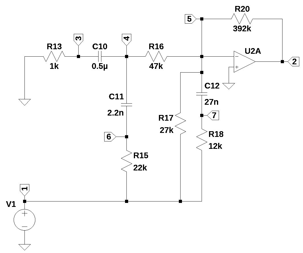
The capacitor, \(C_9\), has been absorbed into \(C_{10}\) in the schematic above in order to reduce the component and node count for the MNA. Since \(C_9\) and \(C_{10}\) are in series, the value of \(C_{10}\) has been adjusted. The capacitor \(C_{13}\) has not been included in the netlist so we can observe the operation of this reactive branch without the zero created at 500 Hz by \(C_{13}\).

reactive_branch_3_4_a_net_list = '''
* Reactive_branch_3b.asc
R13 3 0 1e3
C11 4 6 2.2e-9
R15 6 1 22e3
R17 5 1 27e3
R18 7 1 12e3
C12 5 7 27e-9
R16 5 4 47e3
V1 1 0 1
C10 4 3 0.5e-6
R20 2 5 392e3
*C13 2 5 820e-12
O2A 5 0 2
'''

report, network_df, i_unk_df, A, X, Z = SymMNA.smna(reactive_branch_3_4_a_net_list)

Build the network equations

# Put matrices into SymPy 
X = Matrix(X)
Z = Matrix(Z)

NE_sym = Eq(A*X,Z)

# display the equations
temp = ''
for i in range(shape(NE_sym.lhs)[0]):
    temp += '${:s} = {:s}$<br>'.format(latex(NE_sym.rhs[i]),latex(NE_sym.lhs[i]))
Markdown(temp)

\(0 = I_{V1} + v_{1} \cdot \left(\frac{1}{R_{18}} + \frac{1}{R_{17}} + \frac{1}{R_{15}}\right) - \frac{v_{7}}{R_{18}} - \frac{v_{5}}{R_{17}} - \frac{v_{6}}{R_{15}}\)
\(0 = I_{O2a} + \frac{v_{2}}{R_{20}} - \frac{v_{5}}{R_{20}}\)
\(0 = - C_{10} s v_{4} + v_{3} \left(C_{10} s + \frac{1}{R_{13}}\right)\)
\(0 = - C_{10} s v_{3} - C_{11} s v_{6} + v_{4} \left(C_{10} s + C_{11} s + \frac{1}{R_{16}}\right) - \frac{v_{5}}{R_{16}}\)
\(0 = - C_{12} s v_{7} + v_{5} \left(C_{12} s + \frac{1}{R_{20}} + \frac{1}{R_{17}} + \frac{1}{R_{16}}\right) - \frac{v_{2}}{R_{20}} - \frac{v_{1}}{R_{17}} - \frac{v_{4}}{R_{16}}\)
\(0 = - C_{11} s v_{4} + v_{6} \left(C_{11} s + \frac{1}{R_{15}}\right) - \frac{v_{1}}{R_{15}}\)
\(0 = - C_{12} s v_{5} + v_{7} \left(C_{12} s + \frac{1}{R_{18}}\right) - \frac{v_{1}}{R_{18}}\)
\(V_{1} = v_{1}\)
\(0 = v_{5}\)

Turn the free symbols into SymPy variables and load the element values.

var(str(NE_sym.free_symbols).replace('{','').replace('}',''))
element_values = SymMNA.get_part_values(network_df)

39.3.6.1 Symbolic solution

The network equations can be solved symbolically.

U_sym = solve(NE_sym,X)

Display the node voltages and dependent currents using symbolic notation.

temp = ''
for i in U_sym.keys():
    temp += '${:s} = {:s}$<br>'.format(latex(i),latex(U_sym[i]))

Markdown(temp)

\(v_{1} = V_{1}\)
\(v_{2} = \frac{- C_{10} C_{11} C_{12} R_{13} R_{15} R_{17} R_{20} V_{1} s^{3} - C_{10} C_{11} C_{12} R_{13} R_{15} R_{18} R_{20} V_{1} s^{3} - C_{10} C_{11} C_{12} R_{13} R_{16} R_{17} R_{20} V_{1} s^{3} - C_{10} C_{11} C_{12} R_{13} R_{16} R_{18} R_{20} V_{1} s^{3} - C_{10} C_{11} C_{12} R_{13} R_{17} R_{18} R_{20} V_{1} s^{3} - C_{10} C_{11} C_{12} R_{15} R_{16} R_{17} R_{20} V_{1} s^{3} - C_{10} C_{11} C_{12} R_{15} R_{16} R_{18} R_{20} V_{1} s^{3} - C_{10} C_{11} R_{13} R_{15} R_{20} V_{1} s^{2} - C_{10} C_{11} R_{13} R_{16} R_{20} V_{1} s^{2} - C_{10} C_{11} R_{13} R_{17} R_{20} V_{1} s^{2} - C_{10} C_{11} R_{15} R_{16} R_{20} V_{1} s^{2} - C_{10} C_{12} R_{13} R_{17} R_{20} V_{1} s^{2} - C_{10} C_{12} R_{13} R_{18} R_{20} V_{1} s^{2} - C_{10} C_{12} R_{16} R_{17} R_{20} V_{1} s^{2} - C_{10} C_{12} R_{16} R_{18} R_{20} V_{1} s^{2} - C_{10} R_{13} R_{20} V_{1} s - C_{10} R_{16} R_{20} V_{1} s - C_{11} C_{12} R_{15} R_{17} R_{20} V_{1} s^{2} - C_{11} C_{12} R_{15} R_{18} R_{20} V_{1} s^{2} - C_{11} C_{12} R_{16} R_{17} R_{20} V_{1} s^{2} - C_{11} C_{12} R_{16} R_{18} R_{20} V_{1} s^{2} - C_{11} C_{12} R_{17} R_{18} R_{20} V_{1} s^{2} - C_{11} R_{15} R_{20} V_{1} s - C_{11} R_{16} R_{20} V_{1} s - C_{11} R_{17} R_{20} V_{1} s - C_{12} R_{17} R_{20} V_{1} s - C_{12} R_{18} R_{20} V_{1} s - R_{20} V_{1}}{C_{10} C_{11} C_{12} R_{13} R_{15} R_{17} R_{18} s^{3} + C_{10} C_{11} C_{12} R_{13} R_{16} R_{17} R_{18} s^{3} + C_{10} C_{11} C_{12} R_{15} R_{16} R_{17} R_{18} s^{3} + C_{10} C_{11} R_{13} R_{15} R_{17} s^{2} + C_{10} C_{11} R_{13} R_{16} R_{17} s^{2} + C_{10} C_{11} R_{15} R_{16} R_{17} s^{2} + C_{10} C_{12} R_{13} R_{17} R_{18} s^{2} + C_{10} C_{12} R_{16} R_{17} R_{18} s^{2} + C_{10} R_{13} R_{17} s + C_{10} R_{16} R_{17} s + C_{11} C_{12} R_{15} R_{17} R_{18} s^{2} + C_{11} C_{12} R_{16} R_{17} R_{18} s^{2} + C_{11} R_{15} R_{17} s + C_{11} R_{16} R_{17} s + C_{12} R_{17} R_{18} s + R_{17}}\)
\(v_{3} = \frac{C_{10} C_{11} R_{13} R_{16} V_{1} s^{2}}{C_{10} C_{11} R_{13} R_{15} s^{2} + C_{10} C_{11} R_{13} R_{16} s^{2} + C_{10} C_{11} R_{15} R_{16} s^{2} + C_{10} R_{13} s + C_{10} R_{16} s + C_{11} R_{15} s + C_{11} R_{16} s + 1}\)
\(v_{4} = \frac{C_{10} C_{11} R_{13} R_{16} V_{1} s^{2} + C_{11} R_{16} V_{1} s}{C_{10} C_{11} R_{13} R_{15} s^{2} + C_{10} C_{11} R_{13} R_{16} s^{2} + C_{10} C_{11} R_{15} R_{16} s^{2} + C_{10} R_{13} s + C_{10} R_{16} s + C_{11} R_{15} s + C_{11} R_{16} s + 1}\)
\(v_{5} = 0\)
\(v_{6} = \frac{C_{10} C_{11} R_{13} R_{16} V_{1} s^{2} + C_{10} R_{13} V_{1} s + C_{10} R_{16} V_{1} s + C_{11} R_{16} V_{1} s + V_{1}}{C_{10} C_{11} R_{13} R_{15} s^{2} + C_{10} C_{11} R_{13} R_{16} s^{2} + C_{10} C_{11} R_{15} R_{16} s^{2} + C_{10} R_{13} s + C_{10} R_{16} s + C_{11} R_{15} s + C_{11} R_{16} s + 1}\)
\(v_{7} = \frac{V_{1}}{C_{12} R_{18} s + 1}\)
\(I_{V1} = \frac{- C_{10} C_{11} C_{12} R_{13} R_{15} R_{17} V_{1} s^{3} - C_{10} C_{11} C_{12} R_{13} R_{15} R_{18} V_{1} s^{3} - C_{10} C_{11} C_{12} R_{13} R_{16} R_{17} V_{1} s^{3} - C_{10} C_{11} C_{12} R_{13} R_{16} R_{18} V_{1} s^{3} - C_{10} C_{11} C_{12} R_{13} R_{17} R_{18} V_{1} s^{3} - C_{10} C_{11} C_{12} R_{15} R_{16} R_{17} V_{1} s^{3} - C_{10} C_{11} C_{12} R_{15} R_{16} R_{18} V_{1} s^{3} - C_{10} C_{11} C_{12} R_{16} R_{17} R_{18} V_{1} s^{3} - C_{10} C_{11} R_{13} R_{15} V_{1} s^{2} - C_{10} C_{11} R_{13} R_{16} V_{1} s^{2} - C_{10} C_{11} R_{13} R_{17} V_{1} s^{2} - C_{10} C_{11} R_{15} R_{16} V_{1} s^{2} - C_{10} C_{11} R_{16} R_{17} V_{1} s^{2} - C_{10} C_{12} R_{13} R_{17} V_{1} s^{2} - C_{10} C_{12} R_{13} R_{18} V_{1} s^{2} - C_{10} C_{12} R_{16} R_{17} V_{1} s^{2} - C_{10} C_{12} R_{16} R_{18} V_{1} s^{2} - C_{10} R_{13} V_{1} s - C_{10} R_{16} V_{1} s - C_{11} C_{12} R_{15} R_{17} V_{1} s^{2} - C_{11} C_{12} R_{15} R_{18} V_{1} s^{2} - C_{11} C_{12} R_{16} R_{17} V_{1} s^{2} - C_{11} C_{12} R_{16} R_{18} V_{1} s^{2} - C_{11} C_{12} R_{17} R_{18} V_{1} s^{2} - C_{11} R_{15} V_{1} s - C_{11} R_{16} V_{1} s - C_{11} R_{17} V_{1} s - C_{12} R_{17} V_{1} s - C_{12} R_{18} V_{1} s - V_{1}}{C_{10} C_{11} C_{12} R_{13} R_{15} R_{17} R_{18} s^{3} + C_{10} C_{11} C_{12} R_{13} R_{16} R_{17} R_{18} s^{3} + C_{10} C_{11} C_{12} R_{15} R_{16} R_{17} R_{18} s^{3} + C_{10} C_{11} R_{13} R_{15} R_{17} s^{2} + C_{10} C_{11} R_{13} R_{16} R_{17} s^{2} + C_{10} C_{11} R_{15} R_{16} R_{17} s^{2} + C_{10} C_{12} R_{13} R_{17} R_{18} s^{2} + C_{10} C_{12} R_{16} R_{17} R_{18} s^{2} + C_{10} R_{13} R_{17} s + C_{10} R_{16} R_{17} s + C_{11} C_{12} R_{15} R_{17} R_{18} s^{2} + C_{11} C_{12} R_{16} R_{17} R_{18} s^{2} + C_{11} R_{15} R_{17} s + C_{11} R_{16} R_{17} s + C_{12} R_{17} R_{18} s + R_{17}}\)
\(I_{O2a} = \frac{C_{10} C_{11} C_{12} R_{13} R_{15} R_{17} V_{1} s^{3} + C_{10} C_{11} C_{12} R_{13} R_{15} R_{18} V_{1} s^{3} + C_{10} C_{11} C_{12} R_{13} R_{16} R_{17} V_{1} s^{3} + C_{10} C_{11} C_{12} R_{13} R_{16} R_{18} V_{1} s^{3} + C_{10} C_{11} C_{12} R_{13} R_{17} R_{18} V_{1} s^{3} + C_{10} C_{11} C_{12} R_{15} R_{16} R_{17} V_{1} s^{3} + C_{10} C_{11} C_{12} R_{15} R_{16} R_{18} V_{1} s^{3} + C_{10} C_{11} R_{13} R_{15} V_{1} s^{2} + C_{10} C_{11} R_{13} R_{16} V_{1} s^{2} + C_{10} C_{11} R_{13} R_{17} V_{1} s^{2} + C_{10} C_{11} R_{15} R_{16} V_{1} s^{2} + C_{10} C_{12} R_{13} R_{17} V_{1} s^{2} + C_{10} C_{12} R_{13} R_{18} V_{1} s^{2} + C_{10} C_{12} R_{16} R_{17} V_{1} s^{2} + C_{10} C_{12} R_{16} R_{18} V_{1} s^{2} + C_{10} R_{13} V_{1} s + C_{10} R_{16} V_{1} s + C_{11} C_{12} R_{15} R_{17} V_{1} s^{2} + C_{11} C_{12} R_{15} R_{18} V_{1} s^{2} + C_{11} C_{12} R_{16} R_{17} V_{1} s^{2} + C_{11} C_{12} R_{16} R_{18} V_{1} s^{2} + C_{11} C_{12} R_{17} R_{18} V_{1} s^{2} + C_{11} R_{15} V_{1} s + C_{11} R_{16} V_{1} s + C_{11} R_{17} V_{1} s + C_{12} R_{17} V_{1} s + C_{12} R_{18} V_{1} s + V_{1}}{C_{10} C_{11} C_{12} R_{13} R_{15} R_{17} R_{18} s^{3} + C_{10} C_{11} C_{12} R_{13} R_{16} R_{17} R_{18} s^{3} + C_{10} C_{11} C_{12} R_{15} R_{16} R_{17} R_{18} s^{3} + C_{10} C_{11} R_{13} R_{15} R_{17} s^{2} + C_{10} C_{11} R_{13} R_{16} R_{17} s^{2} + C_{10} C_{11} R_{15} R_{16} R_{17} s^{2} + C_{10} C_{12} R_{13} R_{17} R_{18} s^{2} + C_{10} C_{12} R_{16} R_{17} R_{18} s^{2} + C_{10} R_{13} R_{17} s + C_{10} R_{16} R_{17} s + C_{11} C_{12} R_{15} R_{17} R_{18} s^{2} + C_{11} C_{12} R_{16} R_{17} R_{18} s^{2} + C_{11} R_{15} R_{17} s + C_{11} R_{16} R_{17} s + C_{12} R_{17} R_{18} s + R_{17}}\)

The network transfer function, \(H(s)=\frac {v_2(s)}{v_1(s)}\) is:

H_sym = (U_sym[v2]/U_sym[v1]).cancel()
Markdown('$H(s)={:s}$'.format(latex(H_sym)))

\(H(s)=\frac{- C_{10} C_{11} C_{12} R_{13} R_{15} R_{17} R_{20} s^{3} - C_{10} C_{11} C_{12} R_{13} R_{15} R_{18} R_{20} s^{3} - C_{10} C_{11} C_{12} R_{13} R_{16} R_{17} R_{20} s^{3} - C_{10} C_{11} C_{12} R_{13} R_{16} R_{18} R_{20} s^{3} - C_{10} C_{11} C_{12} R_{13} R_{17} R_{18} R_{20} s^{3} - C_{10} C_{11} C_{12} R_{15} R_{16} R_{17} R_{20} s^{3} - C_{10} C_{11} C_{12} R_{15} R_{16} R_{18} R_{20} s^{3} - C_{10} C_{11} R_{13} R_{15} R_{20} s^{2} - C_{10} C_{11} R_{13} R_{16} R_{20} s^{2} - C_{10} C_{11} R_{13} R_{17} R_{20} s^{2} - C_{10} C_{11} R_{15} R_{16} R_{20} s^{2} - C_{10} C_{12} R_{13} R_{17} R_{20} s^{2} - C_{10} C_{12} R_{13} R_{18} R_{20} s^{2} - C_{10} C_{12} R_{16} R_{17} R_{20} s^{2} - C_{10} C_{12} R_{16} R_{18} R_{20} s^{2} - C_{10} R_{13} R_{20} s - C_{10} R_{16} R_{20} s - C_{11} C_{12} R_{15} R_{17} R_{20} s^{2} - C_{11} C_{12} R_{15} R_{18} R_{20} s^{2} - C_{11} C_{12} R_{16} R_{17} R_{20} s^{2} - C_{11} C_{12} R_{16} R_{18} R_{20} s^{2} - C_{11} C_{12} R_{17} R_{18} R_{20} s^{2} - C_{11} R_{15} R_{20} s - C_{11} R_{16} R_{20} s - C_{11} R_{17} R_{20} s - C_{12} R_{17} R_{20} s - C_{12} R_{18} R_{20} s - R_{20}}{C_{10} C_{11} C_{12} R_{13} R_{15} R_{17} R_{18} s^{3} + C_{10} C_{11} C_{12} R_{13} R_{16} R_{17} R_{18} s^{3} + C_{10} C_{11} C_{12} R_{15} R_{16} R_{17} R_{18} s^{3} + C_{10} C_{11} R_{13} R_{15} R_{17} s^{2} + C_{10} C_{11} R_{13} R_{16} R_{17} s^{2} + C_{10} C_{11} R_{15} R_{16} R_{17} s^{2} + C_{10} C_{12} R_{13} R_{17} R_{18} s^{2} + C_{10} C_{12} R_{16} R_{17} R_{18} s^{2} + C_{10} R_{13} R_{17} s + C_{10} R_{16} R_{17} s + C_{11} C_{12} R_{15} R_{17} R_{18} s^{2} + C_{11} C_{12} R_{16} R_{17} R_{18} s^{2} + C_{11} R_{15} R_{17} s + C_{11} R_{16} R_{17} s + C_{12} R_{17} R_{18} s + R_{17}}\)

The numerator and the denominator are third order polynomials in terms of \(s\). Generally, the order of the dominator is equal to the number of reactive elements in the circuit. The roots of the numerator polynomial are called the zeros of the transfer function and the roots of the denominator are called the poles of the transfer function.

H_sym_num, H_sym_denom = fraction(H_sym,s) #returns numerator and denominator

39.3.6.2 Numerator Polynomial of \(H_{sym}(s)\)

The numerator polynomial is:

Markdown('$N(s)={:s}$'.format(latex(H_sym_num)))

\(N(s)=- C_{10} C_{11} C_{12} R_{13} R_{15} R_{17} R_{20} s^{3} - C_{10} C_{11} C_{12} R_{13} R_{15} R_{18} R_{20} s^{3} - C_{10} C_{11} C_{12} R_{13} R_{16} R_{17} R_{20} s^{3} - C_{10} C_{11} C_{12} R_{13} R_{16} R_{18} R_{20} s^{3} - C_{10} C_{11} C_{12} R_{13} R_{17} R_{18} R_{20} s^{3} - C_{10} C_{11} C_{12} R_{15} R_{16} R_{17} R_{20} s^{3} - C_{10} C_{11} C_{12} R_{15} R_{16} R_{18} R_{20} s^{3} - C_{10} C_{11} R_{13} R_{15} R_{20} s^{2} - C_{10} C_{11} R_{13} R_{16} R_{20} s^{2} - C_{10} C_{11} R_{13} R_{17} R_{20} s^{2} - C_{10} C_{11} R_{15} R_{16} R_{20} s^{2} - C_{10} C_{12} R_{13} R_{17} R_{20} s^{2} - C_{10} C_{12} R_{13} R_{18} R_{20} s^{2} - C_{10} C_{12} R_{16} R_{17} R_{20} s^{2} - C_{10} C_{12} R_{16} R_{18} R_{20} s^{2} - C_{10} R_{13} R_{20} s - C_{10} R_{16} R_{20} s - C_{11} C_{12} R_{15} R_{17} R_{20} s^{2} - C_{11} C_{12} R_{15} R_{18} R_{20} s^{2} - C_{11} C_{12} R_{16} R_{17} R_{20} s^{2} - C_{11} C_{12} R_{16} R_{18} R_{20} s^{2} - C_{11} C_{12} R_{17} R_{18} R_{20} s^{2} - C_{11} R_{15} R_{20} s - C_{11} R_{16} R_{20} s - C_{11} R_{17} R_{20} s - C_{12} R_{17} R_{20} s - C_{12} R_{18} R_{20} s - R_{20}\)

The coefficients of each Laplace term can be equated to the variables \(b_2\), \(b_1\) and \(b_0\) in the expression:

\(b_3s^{3}+b_2s^{2}+b_1s+b_0\)

where \(b_3\), \(b_2\), \(b_1\) and \(b_0\) are:

b3 = H_sym_num.coeff(s**3)
b2 = H_sym_num.coeff(s**2)
b1 = H_sym_num.coeff(s**1)
b0 = (H_sym_num - b1*s*1 - b2*s**2 - b3*s**3).expand()

Markdown('<p>$b_3={:s}$</p><p>$b_2={:s}$</p><p>$b_1={:s}$\
    </p><p>$b_0={:s}$</p>'.format(latex(b3),latex(b2),latex(b1),latex(b0)))

\(b_3=- C_{10} C_{11} C_{12} R_{13} R_{15} R_{17} R_{20} - C_{10} C_{11} C_{12} R_{13} R_{15} R_{18} R_{20} - C_{10} C_{11} C_{12} R_{13} R_{16} R_{17} R_{20} - C_{10} C_{11} C_{12} R_{13} R_{16} R_{18} R_{20} - C_{10} C_{11} C_{12} R_{13} R_{17} R_{18} R_{20} - C_{10} C_{11} C_{12} R_{15} R_{16} R_{17} R_{20} - C_{10} C_{11} C_{12} R_{15} R_{16} R_{18} R_{20}\)

\(b_2=- C_{10} C_{11} R_{13} R_{15} R_{20} - C_{10} C_{11} R_{13} R_{16} R_{20} - C_{10} C_{11} R_{13} R_{17} R_{20} - C_{10} C_{11} R_{15} R_{16} R_{20} - C_{10} C_{12} R_{13} R_{17} R_{20} - C_{10} C_{12} R_{13} R_{18} R_{20} - C_{10} C_{12} R_{16} R_{17} R_{20} - C_{10} C_{12} R_{16} R_{18} R_{20} - C_{11} C_{12} R_{15} R_{17} R_{20} - C_{11} C_{12} R_{15} R_{18} R_{20} - C_{11} C_{12} R_{16} R_{17} R_{20} - C_{11} C_{12} R_{16} R_{18} R_{20} - C_{11} C_{12} R_{17} R_{18} R_{20}\)

\(b_1=- C_{10} R_{13} R_{20} - C_{10} R_{16} R_{20} - C_{11} R_{15} R_{20} - C_{11} R_{16} R_{20} - C_{11} R_{17} R_{20} - C_{12} R_{17} R_{20} - C_{12} R_{18} R_{20}\)

\(b_0=- R_{20}\)

The roots of the numerator polynomial can easily be found with SymPy. This filter has two transmission zeros, which can be found using the solve function on the numerator polynomial.

num_root_sym = solve(H_sym_num,s)

There are three solutions:

Markdown('<p>$z_0={:s}$</p><p>$z_1={:s}$</p><p>$z_2={:s}$</p>'.format(latex(num_root_sym[0]),latex(num_root_sym[1]),latex(num_root_sym[2])))

\(z_0=- \frac{- \frac{3 \left(C_{10} R_{13} + C_{10} R_{16} + C_{11} R_{15} + C_{11} R_{16} + C_{11} R_{17} + C_{12} R_{17} + C_{12} R_{18}\right)}{C_{10} C_{11} C_{12} R_{13} R_{15} R_{17} + C_{10} C_{11} C_{12} R_{13} R_{15} R_{18} + C_{10} C_{11} C_{12} R_{13} R_{16} R_{17} + C_{10} C_{11} C_{12} R_{13} R_{16} R_{18} + C_{10} C_{11} C_{12} R_{13} R_{17} R_{18} + C_{10} C_{11} C_{12} R_{15} R_{16} R_{17} + C_{10} C_{11} C_{12} R_{15} R_{16} R_{18}} + \frac{\left(C_{10} C_{11} R_{13} R_{15} + C_{10} C_{11} R_{13} R_{16} + C_{10} C_{11} R_{13} R_{17} + C_{10} C_{11} R_{15} R_{16} + C_{10} C_{12} R_{13} R_{17} + C_{10} C_{12} R_{13} R_{18} + C_{10} C_{12} R_{16} R_{17} + C_{10} C_{12} R_{16} R_{18} + C_{11} C_{12} R_{15} R_{17} + C_{11} C_{12} R_{15} R_{18} + C_{11} C_{12} R_{16} R_{17} + C_{11} C_{12} R_{16} R_{18} + C_{11} C_{12} R_{17} R_{18}\right)^{2}}{\left(C_{10} C_{11} C_{12} R_{13} R_{15} R_{17} + C_{10} C_{11} C_{12} R_{13} R_{15} R_{18} + C_{10} C_{11} C_{12} R_{13} R_{16} R_{17} + C_{10} C_{11} C_{12} R_{13} R_{16} R_{18} + C_{10} C_{11} C_{12} R_{13} R_{17} R_{18} + C_{10} C_{11} C_{12} R_{15} R_{16} R_{17} + C_{10} C_{11} C_{12} R_{15} R_{16} R_{18}\right)^{2}}}{3 \sqrt[3]{\frac{\sqrt{- 4 \left(- \frac{3 \left(C_{10} R_{13} + C_{10} R_{16} + C_{11} R_{15} + C_{11} R_{16} + C_{11} R_{17} + C_{12} R_{17} + C_{12} R_{18}\right)}{C_{10} C_{11} C_{12} R_{13} R_{15} R_{17} + C_{10} C_{11} C_{12} R_{13} R_{15} R_{18} + C_{10} C_{11} C_{12} R_{13} R_{16} R_{17} + C_{10} C_{11} C_{12} R_{13} R_{16} R_{18} + C_{10} C_{11} C_{12} R_{13} R_{17} R_{18} + C_{10} C_{11} C_{12} R_{15} R_{16} R_{17} + C_{10} C_{11} C_{12} R_{15} R_{16} R_{18}} + \frac{\left(C_{10} C_{11} R_{13} R_{15} + C_{10} C_{11} R_{13} R_{16} + C_{10} C_{11} R_{13} R_{17} + C_{10} C_{11} R_{15} R_{16} + C_{10} C_{12} R_{13} R_{17} + C_{10} C_{12} R_{13} R_{18} + C_{10} C_{12} R_{16} R_{17} + C_{10} C_{12} R_{16} R_{18} + C_{11} C_{12} R_{15} R_{17} + C_{11} C_{12} R_{15} R_{18} + C_{11} C_{12} R_{16} R_{17} + C_{11} C_{12} R_{16} R_{18} + C_{11} C_{12} R_{17} R_{18}\right)^{2}}{\left(C_{10} C_{11} C_{12} R_{13} R_{15} R_{17} + C_{10} C_{11} C_{12} R_{13} R_{15} R_{18} + C_{10} C_{11} C_{12} R_{13} R_{16} R_{17} + C_{10} C_{11} C_{12} R_{13} R_{16} R_{18} + C_{10} C_{11} C_{12} R_{13} R_{17} R_{18} + C_{10} C_{11} C_{12} R_{15} R_{16} R_{17} + C_{10} C_{11} C_{12} R_{15} R_{16} R_{18}\right)^{2}}\right)^{3} + \left(- \frac{9 \left(C_{10} R_{13} + C_{10} R_{16} + C_{11} R_{15} + C_{11} R_{16} + C_{11} R_{17} + C_{12} R_{17} + C_{12} R_{18}\right) \left(C_{10} C_{11} R_{13} R_{15} + C_{10} C_{11} R_{13} R_{16} + C_{10} C_{11} R_{13} R_{17} + C_{10} C_{11} R_{15} R_{16} + C_{10} C_{12} R_{13} R_{17} + C_{10} C_{12} R_{13} R_{18} + C_{10} C_{12} R_{16} R_{17} + C_{10} C_{12} R_{16} R_{18} + C_{11} C_{12} R_{15} R_{17} + C_{11} C_{12} R_{15} R_{18} + C_{11} C_{12} R_{16} R_{17} + C_{11} C_{12} R_{16} R_{18} + C_{11} C_{12} R_{17} R_{18}\right)}{\left(C_{10} C_{11} C_{12} R_{13} R_{15} R_{17} + C_{10} C_{11} C_{12} R_{13} R_{15} R_{18} + C_{10} C_{11} C_{12} R_{13} R_{16} R_{17} + C_{10} C_{11} C_{12} R_{13} R_{16} R_{18} + C_{10} C_{11} C_{12} R_{13} R_{17} R_{18} + C_{10} C_{11} C_{12} R_{15} R_{16} R_{17} + C_{10} C_{11} C_{12} R_{15} R_{16} R_{18}\right)^{2}} + \frac{27}{C_{10} C_{11} C_{12} R_{13} R_{15} R_{17} + C_{10} C_{11} C_{12} R_{13} R_{15} R_{18} + C_{10} C_{11} C_{12} R_{13} R_{16} R_{17} + C_{10} C_{11} C_{12} R_{13} R_{16} R_{18} + C_{10} C_{11} C_{12} R_{13} R_{17} R_{18} + C_{10} C_{11} C_{12} R_{15} R_{16} R_{17} + C_{10} C_{11} C_{12} R_{15} R_{16} R_{18}} + \frac{2 \left(C_{10} C_{11} R_{13} R_{15} + C_{10} C_{11} R_{13} R_{16} + C_{10} C_{11} R_{13} R_{17} + C_{10} C_{11} R_{15} R_{16} + C_{10} C_{12} R_{13} R_{17} + C_{10} C_{12} R_{13} R_{18} + C_{10} C_{12} R_{16} R_{17} + C_{10} C_{12} R_{16} R_{18} + C_{11} C_{12} R_{15} R_{17} + C_{11} C_{12} R_{15} R_{18} + C_{11} C_{12} R_{16} R_{17} + C_{11} C_{12} R_{16} R_{18} + C_{11} C_{12} R_{17} R_{18}\right)^{3}}{\left(C_{10} C_{11} C_{12} R_{13} R_{15} R_{17} + C_{10} C_{11} C_{12} R_{13} R_{15} R_{18} + C_{10} C_{11} C_{12} R_{13} R_{16} R_{17} + C_{10} C_{11} C_{12} R_{13} R_{16} R_{18} + C_{10} C_{11} C_{12} R_{13} R_{17} R_{18} + C_{10} C_{11} C_{12} R_{15} R_{16} R_{17} + C_{10} C_{11} C_{12} R_{15} R_{16} R_{18}\right)^{3}}\right)^{2}}}{2} - \frac{9 \left(C_{10} R_{13} + C_{10} R_{16} + C_{11} R_{15} + C_{11} R_{16} + C_{11} R_{17} + C_{12} R_{17} + C_{12} R_{18}\right) \left(C_{10} C_{11} R_{13} R_{15} + C_{10} C_{11} R_{13} R_{16} + C_{10} C_{11} R_{13} R_{17} + C_{10} C_{11} R_{15} R_{16} + C_{10} C_{12} R_{13} R_{17} + C_{10} C_{12} R_{13} R_{18} + C_{10} C_{12} R_{16} R_{17} + C_{10} C_{12} R_{16} R_{18} + C_{11} C_{12} R_{15} R_{17} + C_{11} C_{12} R_{15} R_{18} + C_{11} C_{12} R_{16} R_{17} + C_{11} C_{12} R_{16} R_{18} + C_{11} C_{12} R_{17} R_{18}\right)}{2 \left(C_{10} C_{11} C_{12} R_{13} R_{15} R_{17} + C_{10} C_{11} C_{12} R_{13} R_{15} R_{18} + C_{10} C_{11} C_{12} R_{13} R_{16} R_{17} + C_{10} C_{11} C_{12} R_{13} R_{16} R_{18} + C_{10} C_{11} C_{12} R_{13} R_{17} R_{18} + C_{10} C_{11} C_{12} R_{15} R_{16} R_{17} + C_{10} C_{11} C_{12} R_{15} R_{16} R_{18}\right)^{2}} + \frac{27}{2 \left(C_{10} C_{11} C_{12} R_{13} R_{15} R_{17} + C_{10} C_{11} C_{12} R_{13} R_{15} R_{18} + C_{10} C_{11} C_{12} R_{13} R_{16} R_{17} + C_{10} C_{11} C_{12} R_{13} R_{16} R_{18} + C_{10} C_{11} C_{12} R_{13} R_{17} R_{18} + C_{10} C_{11} C_{12} R_{15} R_{16} R_{17} + C_{10} C_{11} C_{12} R_{15} R_{16} R_{18}\right)} + \frac{\left(C_{10} C_{11} R_{13} R_{15} + C_{10} C_{11} R_{13} R_{16} + C_{10} C_{11} R_{13} R_{17} + C_{10} C_{11} R_{15} R_{16} + C_{10} C_{12} R_{13} R_{17} + C_{10} C_{12} R_{13} R_{18} + C_{10} C_{12} R_{16} R_{17} + C_{10} C_{12} R_{16} R_{18} + C_{11} C_{12} R_{15} R_{17} + C_{11} C_{12} R_{15} R_{18} + C_{11} C_{12} R_{16} R_{17} + C_{11} C_{12} R_{16} R_{18} + C_{11} C_{12} R_{17} R_{18}\right)^{3}}{\left(C_{10} C_{11} C_{12} R_{13} R_{15} R_{17} + C_{10} C_{11} C_{12} R_{13} R_{15} R_{18} + C_{10} C_{11} C_{12} R_{13} R_{16} R_{17} + C_{10} C_{11} C_{12} R_{13} R_{16} R_{18} + C_{10} C_{11} C_{12} R_{13} R_{17} R_{18} + C_{10} C_{11} C_{12} R_{15} R_{16} R_{17} + C_{10} C_{11} C_{12} R_{15} R_{16} R_{18}\right)^{3}}}} - \frac{\sqrt[3]{\frac{\sqrt{- 4 \left(- \frac{3 \left(C_{10} R_{13} + C_{10} R_{16} + C_{11} R_{15} + C_{11} R_{16} + C_{11} R_{17} + C_{12} R_{17} + C_{12} R_{18}\right)}{C_{10} C_{11} C_{12} R_{13} R_{15} R_{17} + C_{10} C_{11} C_{12} R_{13} R_{15} R_{18} + C_{10} C_{11} C_{12} R_{13} R_{16} R_{17} + C_{10} C_{11} C_{12} R_{13} R_{16} R_{18} + C_{10} C_{11} C_{12} R_{13} R_{17} R_{18} + C_{10} C_{11} C_{12} R_{15} R_{16} R_{17} + C_{10} C_{11} C_{12} R_{15} R_{16} R_{18}} + \frac{\left(C_{10} C_{11} R_{13} R_{15} + C_{10} C_{11} R_{13} R_{16} + C_{10} C_{11} R_{13} R_{17} + C_{10} C_{11} R_{15} R_{16} + C_{10} C_{12} R_{13} R_{17} + C_{10} C_{12} R_{13} R_{18} + C_{10} C_{12} R_{16} R_{17} + C_{10} C_{12} R_{16} R_{18} + C_{11} C_{12} R_{15} R_{17} + C_{11} C_{12} R_{15} R_{18} + C_{11} C_{12} R_{16} R_{17} + C_{11} C_{12} R_{16} R_{18} + C_{11} C_{12} R_{17} R_{18}\right)^{2}}{\left(C_{10} C_{11} C_{12} R_{13} R_{15} R_{17} + C_{10} C_{11} C_{12} R_{13} R_{15} R_{18} + C_{10} C_{11} C_{12} R_{13} R_{16} R_{17} + C_{10} C_{11} C_{12} R_{13} R_{16} R_{18} + C_{10} C_{11} C_{12} R_{13} R_{17} R_{18} + C_{10} C_{11} C_{12} R_{15} R_{16} R_{17} + C_{10} C_{11} C_{12} R_{15} R_{16} R_{18}\right)^{2}}\right)^{3} + \left(- \frac{9 \left(C_{10} R_{13} + C_{10} R_{16} + C_{11} R_{15} + C_{11} R_{16} + C_{11} R_{17} + C_{12} R_{17} + C_{12} R_{18}\right) \left(C_{10} C_{11} R_{13} R_{15} + C_{10} C_{11} R_{13} R_{16} + C_{10} C_{11} R_{13} R_{17} + C_{10} C_{11} R_{15} R_{16} + C_{10} C_{12} R_{13} R_{17} + C_{10} C_{12} R_{13} R_{18} + C_{10} C_{12} R_{16} R_{17} + C_{10} C_{12} R_{16} R_{18} + C_{11} C_{12} R_{15} R_{17} + C_{11} C_{12} R_{15} R_{18} + C_{11} C_{12} R_{16} R_{17} + C_{11} C_{12} R_{16} R_{18} + C_{11} C_{12} R_{17} R_{18}\right)}{\left(C_{10} C_{11} C_{12} R_{13} R_{15} R_{17} + C_{10} C_{11} C_{12} R_{13} R_{15} R_{18} + C_{10} C_{11} C_{12} R_{13} R_{16} R_{17} + C_{10} C_{11} C_{12} R_{13} R_{16} R_{18} + C_{10} C_{11} C_{12} R_{13} R_{17} R_{18} + C_{10} C_{11} C_{12} R_{15} R_{16} R_{17} + C_{10} C_{11} C_{12} R_{15} R_{16} R_{18}\right)^{2}} + \frac{27}{C_{10} C_{11} C_{12} R_{13} R_{15} R_{17} + C_{10} C_{11} C_{12} R_{13} R_{15} R_{18} + C_{10} C_{11} C_{12} R_{13} R_{16} R_{17} + C_{10} C_{11} C_{12} R_{13} R_{16} R_{18} + C_{10} C_{11} C_{12} R_{13} R_{17} R_{18} + C_{10} C_{11} C_{12} R_{15} R_{16} R_{17} + C_{10} C_{11} C_{12} R_{15} R_{16} R_{18}} + \frac{2 \left(C_{10} C_{11} R_{13} R_{15} + C_{10} C_{11} R_{13} R_{16} + C_{10} C_{11} R_{13} R_{17} + C_{10} C_{11} R_{15} R_{16} + C_{10} C_{12} R_{13} R_{17} + C_{10} C_{12} R_{13} R_{18} + C_{10} C_{12} R_{16} R_{17} + C_{10} C_{12} R_{16} R_{18} + C_{11} C_{12} R_{15} R_{17} + C_{11} C_{12} R_{15} R_{18} + C_{11} C_{12} R_{16} R_{17} + C_{11} C_{12} R_{16} R_{18} + C_{11} C_{12} R_{17} R_{18}\right)^{3}}{\left(C_{10} C_{11} C_{12} R_{13} R_{15} R_{17} + C_{10} C_{11} C_{12} R_{13} R_{15} R_{18} + C_{10} C_{11} C_{12} R_{13} R_{16} R_{17} + C_{10} C_{11} C_{12} R_{13} R_{16} R_{18} + C_{10} C_{11} C_{12} R_{13} R_{17} R_{18} + C_{10} C_{11} C_{12} R_{15} R_{16} R_{17} + C_{10} C_{11} C_{12} R_{15} R_{16} R_{18}\right)^{3}}\right)^{2}}}{2} - \frac{9 \left(C_{10} R_{13} + C_{10} R_{16} + C_{11} R_{15} + C_{11} R_{16} + C_{11} R_{17} + C_{12} R_{17} + C_{12} R_{18}\right) \left(C_{10} C_{11} R_{13} R_{15} + C_{10} C_{11} R_{13} R_{16} + C_{10} C_{11} R_{13} R_{17} + C_{10} C_{11} R_{15} R_{16} + C_{10} C_{12} R_{13} R_{17} + C_{10} C_{12} R_{13} R_{18} + C_{10} C_{12} R_{16} R_{17} + C_{10} C_{12} R_{16} R_{18} + C_{11} C_{12} R_{15} R_{17} + C_{11} C_{12} R_{15} R_{18} + C_{11} C_{12} R_{16} R_{17} + C_{11} C_{12} R_{16} R_{18} + C_{11} C_{12} R_{17} R_{18}\right)}{2 \left(C_{10} C_{11} C_{12} R_{13} R_{15} R_{17} + C_{10} C_{11} C_{12} R_{13} R_{15} R_{18} + C_{10} C_{11} C_{12} R_{13} R_{16} R_{17} + C_{10} C_{11} C_{12} R_{13} R_{16} R_{18} + C_{10} C_{11} C_{12} R_{13} R_{17} R_{18} + C_{10} C_{11} C_{12} R_{15} R_{16} R_{17} + C_{10} C_{11} C_{12} R_{15} R_{16} R_{18}\right)^{2}} + \frac{27}{2 \left(C_{10} C_{11} C_{12} R_{13} R_{15} R_{17} + C_{10} C_{11} C_{12} R_{13} R_{15} R_{18} + C_{10} C_{11} C_{12} R_{13} R_{16} R_{17} + C_{10} C_{11} C_{12} R_{13} R_{16} R_{18} + C_{10} C_{11} C_{12} R_{13} R_{17} R_{18} + C_{10} C_{11} C_{12} R_{15} R_{16} R_{17} + C_{10} C_{11} C_{12} R_{15} R_{16} R_{18}\right)} + \frac{\left(C_{10} C_{11} R_{13} R_{15} + C_{10} C_{11} R_{13} R_{16} + C_{10} C_{11} R_{13} R_{17} + C_{10} C_{11} R_{15} R_{16} + C_{10} C_{12} R_{13} R_{17} + C_{10} C_{12} R_{13} R_{18} + C_{10} C_{12} R_{16} R_{17} + C_{10} C_{12} R_{16} R_{18} + C_{11} C_{12} R_{15} R_{17} + C_{11} C_{12} R_{15} R_{18} + C_{11} C_{12} R_{16} R_{17} + C_{11} C_{12} R_{16} R_{18} + C_{11} C_{12} R_{17} R_{18}\right)^{3}}{\left(C_{10} C_{11} C_{12} R_{13} R_{15} R_{17} + C_{10} C_{11} C_{12} R_{13} R_{15} R_{18} + C_{10} C_{11} C_{12} R_{13} R_{16} R_{17} + C_{10} C_{11} C_{12} R_{13} R_{16} R_{18} + C_{10} C_{11} C_{12} R_{13} R_{17} R_{18} + C_{10} C_{11} C_{12} R_{15} R_{16} R_{17} + C_{10} C_{11} C_{12} R_{15} R_{16} R_{18}\right)^{3}}}}{3} - \frac{C_{10} C_{11} R_{13} R_{15} + C_{10} C_{11} R_{13} R_{16} + C_{10} C_{11} R_{13} R_{17} + C_{10} C_{11} R_{15} R_{16} + C_{10} C_{12} R_{13} R_{17} + C_{10} C_{12} R_{13} R_{18} + C_{10} C_{12} R_{16} R_{17} + C_{10} C_{12} R_{16} R_{18} + C_{11} C_{12} R_{15} R_{17} + C_{11} C_{12} R_{15} R_{18} + C_{11} C_{12} R_{16} R_{17} + C_{11} C_{12} R_{16} R_{18} + C_{11} C_{12} R_{17} R_{18}}{3 \left(C_{10} C_{11} C_{12} R_{13} R_{15} R_{17} + C_{10} C_{11} C_{12} R_{13} R_{15} R_{18} + C_{10} C_{11} C_{12} R_{13} R_{16} R_{17} + C_{10} C_{11} C_{12} R_{13} R_{16} R_{18} + C_{10} C_{11} C_{12} R_{13} R_{17} R_{18} + C_{10} C_{11} C_{12} R_{15} R_{16} R_{17} + C_{10} C_{11} C_{12} R_{15} R_{16} R_{18}\right)}\)

\(z_1=- \frac{- \frac{3 \left(C_{10} R_{13} + C_{10} R_{16} + C_{11} R_{15} + C_{11} R_{16} + C_{11} R_{17} + C_{12} R_{17} + C_{12} R_{18}\right)}{C_{10} C_{11} C_{12} R_{13} R_{15} R_{17} + C_{10} C_{11} C_{12} R_{13} R_{15} R_{18} + C_{10} C_{11} C_{12} R_{13} R_{16} R_{17} + C_{10} C_{11} C_{12} R_{13} R_{16} R_{18} + C_{10} C_{11} C_{12} R_{13} R_{17} R_{18} + C_{10} C_{11} C_{12} R_{15} R_{16} R_{17} + C_{10} C_{11} C_{12} R_{15} R_{16} R_{18}} + \frac{\left(C_{10} C_{11} R_{13} R_{15} + C_{10} C_{11} R_{13} R_{16} + C_{10} C_{11} R_{13} R_{17} + C_{10} C_{11} R_{15} R_{16} + C_{10} C_{12} R_{13} R_{17} + C_{10} C_{12} R_{13} R_{18} + C_{10} C_{12} R_{16} R_{17} + C_{10} C_{12} R_{16} R_{18} + C_{11} C_{12} R_{15} R_{17} + C_{11} C_{12} R_{15} R_{18} + C_{11} C_{12} R_{16} R_{17} + C_{11} C_{12} R_{16} R_{18} + C_{11} C_{12} R_{17} R_{18}\right)^{2}}{\left(C_{10} C_{11} C_{12} R_{13} R_{15} R_{17} + C_{10} C_{11} C_{12} R_{13} R_{15} R_{18} + C_{10} C_{11} C_{12} R_{13} R_{16} R_{17} + C_{10} C_{11} C_{12} R_{13} R_{16} R_{18} + C_{10} C_{11} C_{12} R_{13} R_{17} R_{18} + C_{10} C_{11} C_{12} R_{15} R_{16} R_{17} + C_{10} C_{11} C_{12} R_{15} R_{16} R_{18}\right)^{2}}}{3 \left(- \frac{1}{2} - \frac{\sqrt{3} i}{2}\right) \sqrt[3]{\frac{\sqrt{- 4 \left(- \frac{3 \left(C_{10} R_{13} + C_{10} R_{16} + C_{11} R_{15} + C_{11} R_{16} + C_{11} R_{17} + C_{12} R_{17} + C_{12} R_{18}\right)}{C_{10} C_{11} C_{12} R_{13} R_{15} R_{17} + C_{10} C_{11} C_{12} R_{13} R_{15} R_{18} + C_{10} C_{11} C_{12} R_{13} R_{16} R_{17} + C_{10} C_{11} C_{12} R_{13} R_{16} R_{18} + C_{10} C_{11} C_{12} R_{13} R_{17} R_{18} + C_{10} C_{11} C_{12} R_{15} R_{16} R_{17} + C_{10} C_{11} C_{12} R_{15} R_{16} R_{18}} + \frac{\left(C_{10} C_{11} R_{13} R_{15} + C_{10} C_{11} R_{13} R_{16} + C_{10} C_{11} R_{13} R_{17} + C_{10} C_{11} R_{15} R_{16} + C_{10} C_{12} R_{13} R_{17} + C_{10} C_{12} R_{13} R_{18} + C_{10} C_{12} R_{16} R_{17} + C_{10} C_{12} R_{16} R_{18} + C_{11} C_{12} R_{15} R_{17} + C_{11} C_{12} R_{15} R_{18} + C_{11} C_{12} R_{16} R_{17} + C_{11} C_{12} R_{16} R_{18} + C_{11} C_{12} R_{17} R_{18}\right)^{2}}{\left(C_{10} C_{11} C_{12} R_{13} R_{15} R_{17} + C_{10} C_{11} C_{12} R_{13} R_{15} R_{18} + C_{10} C_{11} C_{12} R_{13} R_{16} R_{17} + C_{10} C_{11} C_{12} R_{13} R_{16} R_{18} + C_{10} C_{11} C_{12} R_{13} R_{17} R_{18} + C_{10} C_{11} C_{12} R_{15} R_{16} R_{17} + C_{10} C_{11} C_{12} R_{15} R_{16} R_{18}\right)^{2}}\right)^{3} + \left(- \frac{9 \left(C_{10} R_{13} + C_{10} R_{16} + C_{11} R_{15} + C_{11} R_{16} + C_{11} R_{17} + C_{12} R_{17} + C_{12} R_{18}\right) \left(C_{10} C_{11} R_{13} R_{15} + C_{10} C_{11} R_{13} R_{16} + C_{10} C_{11} R_{13} R_{17} + C_{10} C_{11} R_{15} R_{16} + C_{10} C_{12} R_{13} R_{17} + C_{10} C_{12} R_{13} R_{18} + C_{10} C_{12} R_{16} R_{17} + C_{10} C_{12} R_{16} R_{18} + C_{11} C_{12} R_{15} R_{17} + C_{11} C_{12} R_{15} R_{18} + C_{11} C_{12} R_{16} R_{17} + C_{11} C_{12} R_{16} R_{18} + C_{11} C_{12} R_{17} R_{18}\right)}{\left(C_{10} C_{11} C_{12} R_{13} R_{15} R_{17} + C_{10} C_{11} C_{12} R_{13} R_{15} R_{18} + C_{10} C_{11} C_{12} R_{13} R_{16} R_{17} + C_{10} C_{11} C_{12} R_{13} R_{16} R_{18} + C_{10} C_{11} C_{12} R_{13} R_{17} R_{18} + C_{10} C_{11} C_{12} R_{15} R_{16} R_{17} + C_{10} C_{11} C_{12} R_{15} R_{16} R_{18}\right)^{2}} + \frac{27}{C_{10} C_{11} C_{12} R_{13} R_{15} R_{17} + C_{10} C_{11} C_{12} R_{13} R_{15} R_{18} + C_{10} C_{11} C_{12} R_{13} R_{16} R_{17} + C_{10} C_{11} C_{12} R_{13} R_{16} R_{18} + C_{10} C_{11} C_{12} R_{13} R_{17} R_{18} + C_{10} C_{11} C_{12} R_{15} R_{16} R_{17} + C_{10} C_{11} C_{12} R_{15} R_{16} R_{18}} + \frac{2 \left(C_{10} C_{11} R_{13} R_{15} + C_{10} C_{11} R_{13} R_{16} + C_{10} C_{11} R_{13} R_{17} + C_{10} C_{11} R_{15} R_{16} + C_{10} C_{12} R_{13} R_{17} + C_{10} C_{12} R_{13} R_{18} + C_{10} C_{12} R_{16} R_{17} + C_{10} C_{12} R_{16} R_{18} + C_{11} C_{12} R_{15} R_{17} + C_{11} C_{12} R_{15} R_{18} + C_{11} C_{12} R_{16} R_{17} + C_{11} C_{12} R_{16} R_{18} + C_{11} C_{12} R_{17} R_{18}\right)^{3}}{\left(C_{10} C_{11} C_{12} R_{13} R_{15} R_{17} + C_{10} C_{11} C_{12} R_{13} R_{15} R_{18} + C_{10} C_{11} C_{12} R_{13} R_{16} R_{17} + C_{10} C_{11} C_{12} R_{13} R_{16} R_{18} + C_{10} C_{11} C_{12} R_{13} R_{17} R_{18} + C_{10} C_{11} C_{12} R_{15} R_{16} R_{17} + C_{10} C_{11} C_{12} R_{15} R_{16} R_{18}\right)^{3}}\right)^{2}}}{2} - \frac{9 \left(C_{10} R_{13} + C_{10} R_{16} + C_{11} R_{15} + C_{11} R_{16} + C_{11} R_{17} + C_{12} R_{17} + C_{12} R_{18}\right) \left(C_{10} C_{11} R_{13} R_{15} + C_{10} C_{11} R_{13} R_{16} + C_{10} C_{11} R_{13} R_{17} + C_{10} C_{11} R_{15} R_{16} + C_{10} C_{12} R_{13} R_{17} + C_{10} C_{12} R_{13} R_{18} + C_{10} C_{12} R_{16} R_{17} + C_{10} C_{12} R_{16} R_{18} + C_{11} C_{12} R_{15} R_{17} + C_{11} C_{12} R_{15} R_{18} + C_{11} C_{12} R_{16} R_{17} + C_{11} C_{12} R_{16} R_{18} + C_{11} C_{12} R_{17} R_{18}\right)}{2 \left(C_{10} C_{11} C_{12} R_{13} R_{15} R_{17} + C_{10} C_{11} C_{12} R_{13} R_{15} R_{18} + C_{10} C_{11} C_{12} R_{13} R_{16} R_{17} + C_{10} C_{11} C_{12} R_{13} R_{16} R_{18} + C_{10} C_{11} C_{12} R_{13} R_{17} R_{18} + C_{10} C_{11} C_{12} R_{15} R_{16} R_{17} + C_{10} C_{11} C_{12} R_{15} R_{16} R_{18}\right)^{2}} + \frac{27}{2 \left(C_{10} C_{11} C_{12} R_{13} R_{15} R_{17} + C_{10} C_{11} C_{12} R_{13} R_{15} R_{18} + C_{10} C_{11} C_{12} R_{13} R_{16} R_{17} + C_{10} C_{11} C_{12} R_{13} R_{16} R_{18} + C_{10} C_{11} C_{12} R_{13} R_{17} R_{18} + C_{10} C_{11} C_{12} R_{15} R_{16} R_{17} + C_{10} C_{11} C_{12} R_{15} R_{16} R_{18}\right)} + \frac{\left(C_{10} C_{11} R_{13} R_{15} + C_{10} C_{11} R_{13} R_{16} + C_{10} C_{11} R_{13} R_{17} + C_{10} C_{11} R_{15} R_{16} + C_{10} C_{12} R_{13} R_{17} + C_{10} C_{12} R_{13} R_{18} + C_{10} C_{12} R_{16} R_{17} + C_{10} C_{12} R_{16} R_{18} + C_{11} C_{12} R_{15} R_{17} + C_{11} C_{12} R_{15} R_{18} + C_{11} C_{12} R_{16} R_{17} + C_{11} C_{12} R_{16} R_{18} + C_{11} C_{12} R_{17} R_{18}\right)^{3}}{\left(C_{10} C_{11} C_{12} R_{13} R_{15} R_{17} + C_{10} C_{11} C_{12} R_{13} R_{15} R_{18} + C_{10} C_{11} C_{12} R_{13} R_{16} R_{17} + C_{10} C_{11} C_{12} R_{13} R_{16} R_{18} + C_{10} C_{11} C_{12} R_{13} R_{17} R_{18} + C_{10} C_{11} C_{12} R_{15} R_{16} R_{17} + C_{10} C_{11} C_{12} R_{15} R_{16} R_{18}\right)^{3}}}} - \frac{\left(- \frac{1}{2} - \frac{\sqrt{3} i}{2}\right) \sqrt[3]{\frac{\sqrt{- 4 \left(- \frac{3 \left(C_{10} R_{13} + C_{10} R_{16} + C_{11} R_{15} + C_{11} R_{16} + C_{11} R_{17} + C_{12} R_{17} + C_{12} R_{18}\right)}{C_{10} C_{11} C_{12} R_{13} R_{15} R_{17} + C_{10} C_{11} C_{12} R_{13} R_{15} R_{18} + C_{10} C_{11} C_{12} R_{13} R_{16} R_{17} + C_{10} C_{11} C_{12} R_{13} R_{16} R_{18} + C_{10} C_{11} C_{12} R_{13} R_{17} R_{18} + C_{10} C_{11} C_{12} R_{15} R_{16} R_{17} + C_{10} C_{11} C_{12} R_{15} R_{16} R_{18}} + \frac{\left(C_{10} C_{11} R_{13} R_{15} + C_{10} C_{11} R_{13} R_{16} + C_{10} C_{11} R_{13} R_{17} + C_{10} C_{11} R_{15} R_{16} + C_{10} C_{12} R_{13} R_{17} + C_{10} C_{12} R_{13} R_{18} + C_{10} C_{12} R_{16} R_{17} + C_{10} C_{12} R_{16} R_{18} + C_{11} C_{12} R_{15} R_{17} + C_{11} C_{12} R_{15} R_{18} + C_{11} C_{12} R_{16} R_{17} + C_{11} C_{12} R_{16} R_{18} + C_{11} C_{12} R_{17} R_{18}\right)^{2}}{\left(C_{10} C_{11} C_{12} R_{13} R_{15} R_{17} + C_{10} C_{11} C_{12} R_{13} R_{15} R_{18} + C_{10} C_{11} C_{12} R_{13} R_{16} R_{17} + C_{10} C_{11} C_{12} R_{13} R_{16} R_{18} + C_{10} C_{11} C_{12} R_{13} R_{17} R_{18} + C_{10} C_{11} C_{12} R_{15} R_{16} R_{17} + C_{10} C_{11} C_{12} R_{15} R_{16} R_{18}\right)^{2}}\right)^{3} + \left(- \frac{9 \left(C_{10} R_{13} + C_{10} R_{16} + C_{11} R_{15} + C_{11} R_{16} + C_{11} R_{17} + C_{12} R_{17} + C_{12} R_{18}\right) \left(C_{10} C_{11} R_{13} R_{15} + C_{10} C_{11} R_{13} R_{16} + C_{10} C_{11} R_{13} R_{17} + C_{10} C_{11} R_{15} R_{16} + C_{10} C_{12} R_{13} R_{17} + C_{10} C_{12} R_{13} R_{18} + C_{10} C_{12} R_{16} R_{17} + C_{10} C_{12} R_{16} R_{18} + C_{11} C_{12} R_{15} R_{17} + C_{11} C_{12} R_{15} R_{18} + C_{11} C_{12} R_{16} R_{17} + C_{11} C_{12} R_{16} R_{18} + C_{11} C_{12} R_{17} R_{18}\right)}{\left(C_{10} C_{11} C_{12} R_{13} R_{15} R_{17} + C_{10} C_{11} C_{12} R_{13} R_{15} R_{18} + C_{10} C_{11} C_{12} R_{13} R_{16} R_{17} + C_{10} C_{11} C_{12} R_{13} R_{16} R_{18} + C_{10} C_{11} C_{12} R_{13} R_{17} R_{18} + C_{10} C_{11} C_{12} R_{15} R_{16} R_{17} + C_{10} C_{11} C_{12} R_{15} R_{16} R_{18}\right)^{2}} + \frac{27}{C_{10} C_{11} C_{12} R_{13} R_{15} R_{17} + C_{10} C_{11} C_{12} R_{13} R_{15} R_{18} + C_{10} C_{11} C_{12} R_{13} R_{16} R_{17} + C_{10} C_{11} C_{12} R_{13} R_{16} R_{18} + C_{10} C_{11} C_{12} R_{13} R_{17} R_{18} + C_{10} C_{11} C_{12} R_{15} R_{16} R_{17} + C_{10} C_{11} C_{12} R_{15} R_{16} R_{18}} + \frac{2 \left(C_{10} C_{11} R_{13} R_{15} + C_{10} C_{11} R_{13} R_{16} + C_{10} C_{11} R_{13} R_{17} + C_{10} C_{11} R_{15} R_{16} + C_{10} C_{12} R_{13} R_{17} + C_{10} C_{12} R_{13} R_{18} + C_{10} C_{12} R_{16} R_{17} + C_{10} C_{12} R_{16} R_{18} + C_{11} C_{12} R_{15} R_{17} + C_{11} C_{12} R_{15} R_{18} + C_{11} C_{12} R_{16} R_{17} + C_{11} C_{12} R_{16} R_{18} + C_{11} C_{12} R_{17} R_{18}\right)^{3}}{\left(C_{10} C_{11} C_{12} R_{13} R_{15} R_{17} + C_{10} C_{11} C_{12} R_{13} R_{15} R_{18} + C_{10} C_{11} C_{12} R_{13} R_{16} R_{17} + C_{10} C_{11} C_{12} R_{13} R_{16} R_{18} + C_{10} C_{11} C_{12} R_{13} R_{17} R_{18} + C_{10} C_{11} C_{12} R_{15} R_{16} R_{17} + C_{10} C_{11} C_{12} R_{15} R_{16} R_{18}\right)^{3}}\right)^{2}}}{2} - \frac{9 \left(C_{10} R_{13} + C_{10} R_{16} + C_{11} R_{15} + C_{11} R_{16} + C_{11} R_{17} + C_{12} R_{17} + C_{12} R_{18}\right) \left(C_{10} C_{11} R_{13} R_{15} + C_{10} C_{11} R_{13} R_{16} + C_{10} C_{11} R_{13} R_{17} + C_{10} C_{11} R_{15} R_{16} + C_{10} C_{12} R_{13} R_{17} + C_{10} C_{12} R_{13} R_{18} + C_{10} C_{12} R_{16} R_{17} + C_{10} C_{12} R_{16} R_{18} + C_{11} C_{12} R_{15} R_{17} + C_{11} C_{12} R_{15} R_{18} + C_{11} C_{12} R_{16} R_{17} + C_{11} C_{12} R_{16} R_{18} + C_{11} C_{12} R_{17} R_{18}\right)}{2 \left(C_{10} C_{11} C_{12} R_{13} R_{15} R_{17} + C_{10} C_{11} C_{12} R_{13} R_{15} R_{18} + C_{10} C_{11} C_{12} R_{13} R_{16} R_{17} + C_{10} C_{11} C_{12} R_{13} R_{16} R_{18} + C_{10} C_{11} C_{12} R_{13} R_{17} R_{18} + C_{10} C_{11} C_{12} R_{15} R_{16} R_{17} + C_{10} C_{11} C_{12} R_{15} R_{16} R_{18}\right)^{2}} + \frac{27}{2 \left(C_{10} C_{11} C_{12} R_{13} R_{15} R_{17} + C_{10} C_{11} C_{12} R_{13} R_{15} R_{18} + C_{10} C_{11} C_{12} R_{13} R_{16} R_{17} + C_{10} C_{11} C_{12} R_{13} R_{16} R_{18} + C_{10} C_{11} C_{12} R_{13} R_{17} R_{18} + C_{10} C_{11} C_{12} R_{15} R_{16} R_{17} + C_{10} C_{11} C_{12} R_{15} R_{16} R_{18}\right)} + \frac{\left(C_{10} C_{11} R_{13} R_{15} + C_{10} C_{11} R_{13} R_{16} + C_{10} C_{11} R_{13} R_{17} + C_{10} C_{11} R_{15} R_{16} + C_{10} C_{12} R_{13} R_{17} + C_{10} C_{12} R_{13} R_{18} + C_{10} C_{12} R_{16} R_{17} + C_{10} C_{12} R_{16} R_{18} + C_{11} C_{12} R_{15} R_{17} + C_{11} C_{12} R_{15} R_{18} + C_{11} C_{12} R_{16} R_{17} + C_{11} C_{12} R_{16} R_{18} + C_{11} C_{12} R_{17} R_{18}\right)^{3}}{\left(C_{10} C_{11} C_{12} R_{13} R_{15} R_{17} + C_{10} C_{11} C_{12} R_{13} R_{15} R_{18} + C_{10} C_{11} C_{12} R_{13} R_{16} R_{17} + C_{10} C_{11} C_{12} R_{13} R_{16} R_{18} + C_{10} C_{11} C_{12} R_{13} R_{17} R_{18} + C_{10} C_{11} C_{12} R_{15} R_{16} R_{17} + C_{10} C_{11} C_{12} R_{15} R_{16} R_{18}\right)^{3}}}}{3} - \frac{C_{10} C_{11} R_{13} R_{15} + C_{10} C_{11} R_{13} R_{16} + C_{10} C_{11} R_{13} R_{17} + C_{10} C_{11} R_{15} R_{16} + C_{10} C_{12} R_{13} R_{17} + C_{10} C_{12} R_{13} R_{18} + C_{10} C_{12} R_{16} R_{17} + C_{10} C_{12} R_{16} R_{18} + C_{11} C_{12} R_{15} R_{17} + C_{11} C_{12} R_{15} R_{18} + C_{11} C_{12} R_{16} R_{17} + C_{11} C_{12} R_{16} R_{18} + C_{11} C_{12} R_{17} R_{18}}{3 \left(C_{10} C_{11} C_{12} R_{13} R_{15} R_{17} + C_{10} C_{11} C_{12} R_{13} R_{15} R_{18} + C_{10} C_{11} C_{12} R_{13} R_{16} R_{17} + C_{10} C_{11} C_{12} R_{13} R_{16} R_{18} + C_{10} C_{11} C_{12} R_{13} R_{17} R_{18} + C_{10} C_{11} C_{12} R_{15} R_{16} R_{17} + C_{10} C_{11} C_{12} R_{15} R_{16} R_{18}\right)}\)

\(z_2=- \frac{- \frac{3 \left(C_{10} R_{13} + C_{10} R_{16} + C_{11} R_{15} + C_{11} R_{16} + C_{11} R_{17} + C_{12} R_{17} + C_{12} R_{18}\right)}{C_{10} C_{11} C_{12} R_{13} R_{15} R_{17} + C_{10} C_{11} C_{12} R_{13} R_{15} R_{18} + C_{10} C_{11} C_{12} R_{13} R_{16} R_{17} + C_{10} C_{11} C_{12} R_{13} R_{16} R_{18} + C_{10} C_{11} C_{12} R_{13} R_{17} R_{18} + C_{10} C_{11} C_{12} R_{15} R_{16} R_{17} + C_{10} C_{11} C_{12} R_{15} R_{16} R_{18}} + \frac{\left(C_{10} C_{11} R_{13} R_{15} + C_{10} C_{11} R_{13} R_{16} + C_{10} C_{11} R_{13} R_{17} + C_{10} C_{11} R_{15} R_{16} + C_{10} C_{12} R_{13} R_{17} + C_{10} C_{12} R_{13} R_{18} + C_{10} C_{12} R_{16} R_{17} + C_{10} C_{12} R_{16} R_{18} + C_{11} C_{12} R_{15} R_{17} + C_{11} C_{12} R_{15} R_{18} + C_{11} C_{12} R_{16} R_{17} + C_{11} C_{12} R_{16} R_{18} + C_{11} C_{12} R_{17} R_{18}\right)^{2}}{\left(C_{10} C_{11} C_{12} R_{13} R_{15} R_{17} + C_{10} C_{11} C_{12} R_{13} R_{15} R_{18} + C_{10} C_{11} C_{12} R_{13} R_{16} R_{17} + C_{10} C_{11} C_{12} R_{13} R_{16} R_{18} + C_{10} C_{11} C_{12} R_{13} R_{17} R_{18} + C_{10} C_{11} C_{12} R_{15} R_{16} R_{17} + C_{10} C_{11} C_{12} R_{15} R_{16} R_{18}\right)^{2}}}{3 \left(- \frac{1}{2} + \frac{\sqrt{3} i}{2}\right) \sqrt[3]{\frac{\sqrt{- 4 \left(- \frac{3 \left(C_{10} R_{13} + C_{10} R_{16} + C_{11} R_{15} + C_{11} R_{16} + C_{11} R_{17} + C_{12} R_{17} + C_{12} R_{18}\right)}{C_{10} C_{11} C_{12} R_{13} R_{15} R_{17} + C_{10} C_{11} C_{12} R_{13} R_{15} R_{18} + C_{10} C_{11} C_{12} R_{13} R_{16} R_{17} + C_{10} C_{11} C_{12} R_{13} R_{16} R_{18} + C_{10} C_{11} C_{12} R_{13} R_{17} R_{18} + C_{10} C_{11} C_{12} R_{15} R_{16} R_{17} + C_{10} C_{11} C_{12} R_{15} R_{16} R_{18}} + \frac{\left(C_{10} C_{11} R_{13} R_{15} + C_{10} C_{11} R_{13} R_{16} + C_{10} C_{11} R_{13} R_{17} + C_{10} C_{11} R_{15} R_{16} + C_{10} C_{12} R_{13} R_{17} + C_{10} C_{12} R_{13} R_{18} + C_{10} C_{12} R_{16} R_{17} + C_{10} C_{12} R_{16} R_{18} + C_{11} C_{12} R_{15} R_{17} + C_{11} C_{12} R_{15} R_{18} + C_{11} C_{12} R_{16} R_{17} + C_{11} C_{12} R_{16} R_{18} + C_{11} C_{12} R_{17} R_{18}\right)^{2}}{\left(C_{10} C_{11} C_{12} R_{13} R_{15} R_{17} + C_{10} C_{11} C_{12} R_{13} R_{15} R_{18} + C_{10} C_{11} C_{12} R_{13} R_{16} R_{17} + C_{10} C_{11} C_{12} R_{13} R_{16} R_{18} + C_{10} C_{11} C_{12} R_{13} R_{17} R_{18} + C_{10} C_{11} C_{12} R_{15} R_{16} R_{17} + C_{10} C_{11} C_{12} R_{15} R_{16} R_{18}\right)^{2}}\right)^{3} + \left(- \frac{9 \left(C_{10} R_{13} + C_{10} R_{16} + C_{11} R_{15} + C_{11} R_{16} + C_{11} R_{17} + C_{12} R_{17} + C_{12} R_{18}\right) \left(C_{10} C_{11} R_{13} R_{15} + C_{10} C_{11} R_{13} R_{16} + C_{10} C_{11} R_{13} R_{17} + C_{10} C_{11} R_{15} R_{16} + C_{10} C_{12} R_{13} R_{17} + C_{10} C_{12} R_{13} R_{18} + C_{10} C_{12} R_{16} R_{17} + C_{10} C_{12} R_{16} R_{18} + C_{11} C_{12} R_{15} R_{17} + C_{11} C_{12} R_{15} R_{18} + C_{11} C_{12} R_{16} R_{17} + C_{11} C_{12} R_{16} R_{18} + C_{11} C_{12} R_{17} R_{18}\right)}{\left(C_{10} C_{11} C_{12} R_{13} R_{15} R_{17} + C_{10} C_{11} C_{12} R_{13} R_{15} R_{18} + C_{10} C_{11} C_{12} R_{13} R_{16} R_{17} + C_{10} C_{11} C_{12} R_{13} R_{16} R_{18} + C_{10} C_{11} C_{12} R_{13} R_{17} R_{18} + C_{10} C_{11} C_{12} R_{15} R_{16} R_{17} + C_{10} C_{11} C_{12} R_{15} R_{16} R_{18}\right)^{2}} + \frac{27}{C_{10} C_{11} C_{12} R_{13} R_{15} R_{17} + C_{10} C_{11} C_{12} R_{13} R_{15} R_{18} + C_{10} C_{11} C_{12} R_{13} R_{16} R_{17} + C_{10} C_{11} C_{12} R_{13} R_{16} R_{18} + C_{10} C_{11} C_{12} R_{13} R_{17} R_{18} + C_{10} C_{11} C_{12} R_{15} R_{16} R_{17} + C_{10} C_{11} C_{12} R_{15} R_{16} R_{18}} + \frac{2 \left(C_{10} C_{11} R_{13} R_{15} + C_{10} C_{11} R_{13} R_{16} + C_{10} C_{11} R_{13} R_{17} + C_{10} C_{11} R_{15} R_{16} + C_{10} C_{12} R_{13} R_{17} + C_{10} C_{12} R_{13} R_{18} + C_{10} C_{12} R_{16} R_{17} + C_{10} C_{12} R_{16} R_{18} + C_{11} C_{12} R_{15} R_{17} + C_{11} C_{12} R_{15} R_{18} + C_{11} C_{12} R_{16} R_{17} + C_{11} C_{12} R_{16} R_{18} + C_{11} C_{12} R_{17} R_{18}\right)^{3}}{\left(C_{10} C_{11} C_{12} R_{13} R_{15} R_{17} + C_{10} C_{11} C_{12} R_{13} R_{15} R_{18} + C_{10} C_{11} C_{12} R_{13} R_{16} R_{17} + C_{10} C_{11} C_{12} R_{13} R_{16} R_{18} + C_{10} C_{11} C_{12} R_{13} R_{17} R_{18} + C_{10} C_{11} C_{12} R_{15} R_{16} R_{17} + C_{10} C_{11} C_{12} R_{15} R_{16} R_{18}\right)^{3}}\right)^{2}}}{2} - \frac{9 \left(C_{10} R_{13} + C_{10} R_{16} + C_{11} R_{15} + C_{11} R_{16} + C_{11} R_{17} + C_{12} R_{17} + C_{12} R_{18}\right) \left(C_{10} C_{11} R_{13} R_{15} + C_{10} C_{11} R_{13} R_{16} + C_{10} C_{11} R_{13} R_{17} + C_{10} C_{11} R_{15} R_{16} + C_{10} C_{12} R_{13} R_{17} + C_{10} C_{12} R_{13} R_{18} + C_{10} C_{12} R_{16} R_{17} + C_{10} C_{12} R_{16} R_{18} + C_{11} C_{12} R_{15} R_{17} + C_{11} C_{12} R_{15} R_{18} + C_{11} C_{12} R_{16} R_{17} + C_{11} C_{12} R_{16} R_{18} + C_{11} C_{12} R_{17} R_{18}\right)}{2 \left(C_{10} C_{11} C_{12} R_{13} R_{15} R_{17} + C_{10} C_{11} C_{12} R_{13} R_{15} R_{18} + C_{10} C_{11} C_{12} R_{13} R_{16} R_{17} + C_{10} C_{11} C_{12} R_{13} R_{16} R_{18} + C_{10} C_{11} C_{12} R_{13} R_{17} R_{18} + C_{10} C_{11} C_{12} R_{15} R_{16} R_{17} + C_{10} C_{11} C_{12} R_{15} R_{16} R_{18}\right)^{2}} + \frac{27}{2 \left(C_{10} C_{11} C_{12} R_{13} R_{15} R_{17} + C_{10} C_{11} C_{12} R_{13} R_{15} R_{18} + C_{10} C_{11} C_{12} R_{13} R_{16} R_{17} + C_{10} C_{11} C_{12} R_{13} R_{16} R_{18} + C_{10} C_{11} C_{12} R_{13} R_{17} R_{18} + C_{10} C_{11} C_{12} R_{15} R_{16} R_{17} + C_{10} C_{11} C_{12} R_{15} R_{16} R_{18}\right)} + \frac{\left(C_{10} C_{11} R_{13} R_{15} + C_{10} C_{11} R_{13} R_{16} + C_{10} C_{11} R_{13} R_{17} + C_{10} C_{11} R_{15} R_{16} + C_{10} C_{12} R_{13} R_{17} + C_{10} C_{12} R_{13} R_{18} + C_{10} C_{12} R_{16} R_{17} + C_{10} C_{12} R_{16} R_{18} + C_{11} C_{12} R_{15} R_{17} + C_{11} C_{12} R_{15} R_{18} + C_{11} C_{12} R_{16} R_{17} + C_{11} C_{12} R_{16} R_{18} + C_{11} C_{12} R_{17} R_{18}\right)^{3}}{\left(C_{10} C_{11} C_{12} R_{13} R_{15} R_{17} + C_{10} C_{11} C_{12} R_{13} R_{15} R_{18} + C_{10} C_{11} C_{12} R_{13} R_{16} R_{17} + C_{10} C_{11} C_{12} R_{13} R_{16} R_{18} + C_{10} C_{11} C_{12} R_{13} R_{17} R_{18} + C_{10} C_{11} C_{12} R_{15} R_{16} R_{17} + C_{10} C_{11} C_{12} R_{15} R_{16} R_{18}\right)^{3}}}} - \frac{\left(- \frac{1}{2} + \frac{\sqrt{3} i}{2}\right) \sqrt[3]{\frac{\sqrt{- 4 \left(- \frac{3 \left(C_{10} R_{13} + C_{10} R_{16} + C_{11} R_{15} + C_{11} R_{16} + C_{11} R_{17} + C_{12} R_{17} + C_{12} R_{18}\right)}{C_{10} C_{11} C_{12} R_{13} R_{15} R_{17} + C_{10} C_{11} C_{12} R_{13} R_{15} R_{18} + C_{10} C_{11} C_{12} R_{13} R_{16} R_{17} + C_{10} C_{11} C_{12} R_{13} R_{16} R_{18} + C_{10} C_{11} C_{12} R_{13} R_{17} R_{18} + C_{10} C_{11} C_{12} R_{15} R_{16} R_{17} + C_{10} C_{11} C_{12} R_{15} R_{16} R_{18}} + \frac{\left(C_{10} C_{11} R_{13} R_{15} + C_{10} C_{11} R_{13} R_{16} + C_{10} C_{11} R_{13} R_{17} + C_{10} C_{11} R_{15} R_{16} + C_{10} C_{12} R_{13} R_{17} + C_{10} C_{12} R_{13} R_{18} + C_{10} C_{12} R_{16} R_{17} + C_{10} C_{12} R_{16} R_{18} + C_{11} C_{12} R_{15} R_{17} + C_{11} C_{12} R_{15} R_{18} + C_{11} C_{12} R_{16} R_{17} + C_{11} C_{12} R_{16} R_{18} + C_{11} C_{12} R_{17} R_{18}\right)^{2}}{\left(C_{10} C_{11} C_{12} R_{13} R_{15} R_{17} + C_{10} C_{11} C_{12} R_{13} R_{15} R_{18} + C_{10} C_{11} C_{12} R_{13} R_{16} R_{17} + C_{10} C_{11} C_{12} R_{13} R_{16} R_{18} + C_{10} C_{11} C_{12} R_{13} R_{17} R_{18} + C_{10} C_{11} C_{12} R_{15} R_{16} R_{17} + C_{10} C_{11} C_{12} R_{15} R_{16} R_{18}\right)^{2}}\right)^{3} + \left(- \frac{9 \left(C_{10} R_{13} + C_{10} R_{16} + C_{11} R_{15} + C_{11} R_{16} + C_{11} R_{17} + C_{12} R_{17} + C_{12} R_{18}\right) \left(C_{10} C_{11} R_{13} R_{15} + C_{10} C_{11} R_{13} R_{16} + C_{10} C_{11} R_{13} R_{17} + C_{10} C_{11} R_{15} R_{16} + C_{10} C_{12} R_{13} R_{17} + C_{10} C_{12} R_{13} R_{18} + C_{10} C_{12} R_{16} R_{17} + C_{10} C_{12} R_{16} R_{18} + C_{11} C_{12} R_{15} R_{17} + C_{11} C_{12} R_{15} R_{18} + C_{11} C_{12} R_{16} R_{17} + C_{11} C_{12} R_{16} R_{18} + C_{11} C_{12} R_{17} R_{18}\right)}{\left(C_{10} C_{11} C_{12} R_{13} R_{15} R_{17} + C_{10} C_{11} C_{12} R_{13} R_{15} R_{18} + C_{10} C_{11} C_{12} R_{13} R_{16} R_{17} + C_{10} C_{11} C_{12} R_{13} R_{16} R_{18} + C_{10} C_{11} C_{12} R_{13} R_{17} R_{18} + C_{10} C_{11} C_{12} R_{15} R_{16} R_{17} + C_{10} C_{11} C_{12} R_{15} R_{16} R_{18}\right)^{2}} + \frac{27}{C_{10} C_{11} C_{12} R_{13} R_{15} R_{17} + C_{10} C_{11} C_{12} R_{13} R_{15} R_{18} + C_{10} C_{11} C_{12} R_{13} R_{16} R_{17} + C_{10} C_{11} C_{12} R_{13} R_{16} R_{18} + C_{10} C_{11} C_{12} R_{13} R_{17} R_{18} + C_{10} C_{11} C_{12} R_{15} R_{16} R_{17} + C_{10} C_{11} C_{12} R_{15} R_{16} R_{18}} + \frac{2 \left(C_{10} C_{11} R_{13} R_{15} + C_{10} C_{11} R_{13} R_{16} + C_{10} C_{11} R_{13} R_{17} + C_{10} C_{11} R_{15} R_{16} + C_{10} C_{12} R_{13} R_{17} + C_{10} C_{12} R_{13} R_{18} + C_{10} C_{12} R_{16} R_{17} + C_{10} C_{12} R_{16} R_{18} + C_{11} C_{12} R_{15} R_{17} + C_{11} C_{12} R_{15} R_{18} + C_{11} C_{12} R_{16} R_{17} + C_{11} C_{12} R_{16} R_{18} + C_{11} C_{12} R_{17} R_{18}\right)^{3}}{\left(C_{10} C_{11} C_{12} R_{13} R_{15} R_{17} + C_{10} C_{11} C_{12} R_{13} R_{15} R_{18} + C_{10} C_{11} C_{12} R_{13} R_{16} R_{17} + C_{10} C_{11} C_{12} R_{13} R_{16} R_{18} + C_{10} C_{11} C_{12} R_{13} R_{17} R_{18} + C_{10} C_{11} C_{12} R_{15} R_{16} R_{17} + C_{10} C_{11} C_{12} R_{15} R_{16} R_{18}\right)^{3}}\right)^{2}}}{2} - \frac{9 \left(C_{10} R_{13} + C_{10} R_{16} + C_{11} R_{15} + C_{11} R_{16} + C_{11} R_{17} + C_{12} R_{17} + C_{12} R_{18}\right) \left(C_{10} C_{11} R_{13} R_{15} + C_{10} C_{11} R_{13} R_{16} + C_{10} C_{11} R_{13} R_{17} + C_{10} C_{11} R_{15} R_{16} + C_{10} C_{12} R_{13} R_{17} + C_{10} C_{12} R_{13} R_{18} + C_{10} C_{12} R_{16} R_{17} + C_{10} C_{12} R_{16} R_{18} + C_{11} C_{12} R_{15} R_{17} + C_{11} C_{12} R_{15} R_{18} + C_{11} C_{12} R_{16} R_{17} + C_{11} C_{12} R_{16} R_{18} + C_{11} C_{12} R_{17} R_{18}\right)}{2 \left(C_{10} C_{11} C_{12} R_{13} R_{15} R_{17} + C_{10} C_{11} C_{12} R_{13} R_{15} R_{18} + C_{10} C_{11} C_{12} R_{13} R_{16} R_{17} + C_{10} C_{11} C_{12} R_{13} R_{16} R_{18} + C_{10} C_{11} C_{12} R_{13} R_{17} R_{18} + C_{10} C_{11} C_{12} R_{15} R_{16} R_{17} + C_{10} C_{11} C_{12} R_{15} R_{16} R_{18}\right)^{2}} + \frac{27}{2 \left(C_{10} C_{11} C_{12} R_{13} R_{15} R_{17} + C_{10} C_{11} C_{12} R_{13} R_{15} R_{18} + C_{10} C_{11} C_{12} R_{13} R_{16} R_{17} + C_{10} C_{11} C_{12} R_{13} R_{16} R_{18} + C_{10} C_{11} C_{12} R_{13} R_{17} R_{18} + C_{10} C_{11} C_{12} R_{15} R_{16} R_{17} + C_{10} C_{11} C_{12} R_{15} R_{16} R_{18}\right)} + \frac{\left(C_{10} C_{11} R_{13} R_{15} + C_{10} C_{11} R_{13} R_{16} + C_{10} C_{11} R_{13} R_{17} + C_{10} C_{11} R_{15} R_{16} + C_{10} C_{12} R_{13} R_{17} + C_{10} C_{12} R_{13} R_{18} + C_{10} C_{12} R_{16} R_{17} + C_{10} C_{12} R_{16} R_{18} + C_{11} C_{12} R_{15} R_{17} + C_{11} C_{12} R_{15} R_{18} + C_{11} C_{12} R_{16} R_{17} + C_{11} C_{12} R_{16} R_{18} + C_{11} C_{12} R_{17} R_{18}\right)^{3}}{\left(C_{10} C_{11} C_{12} R_{13} R_{15} R_{17} + C_{10} C_{11} C_{12} R_{13} R_{15} R_{18} + C_{10} C_{11} C_{12} R_{13} R_{16} R_{17} + C_{10} C_{11} C_{12} R_{13} R_{16} R_{18} + C_{10} C_{11} C_{12} R_{13} R_{17} R_{18} + C_{10} C_{11} C_{12} R_{15} R_{16} R_{17} + C_{10} C_{11} C_{12} R_{15} R_{16} R_{18}\right)^{3}}}}{3} - \frac{C_{10} C_{11} R_{13} R_{15} + C_{10} C_{11} R_{13} R_{16} + C_{10} C_{11} R_{13} R_{17} + C_{10} C_{11} R_{15} R_{16} + C_{10} C_{12} R_{13} R_{17} + C_{10} C_{12} R_{13} R_{18} + C_{10} C_{12} R_{16} R_{17} + C_{10} C_{12} R_{16} R_{18} + C_{11} C_{12} R_{15} R_{17} + C_{11} C_{12} R_{15} R_{18} + C_{11} C_{12} R_{16} R_{17} + C_{11} C_{12} R_{16} R_{18} + C_{11} C_{12} R_{17} R_{18}}{3 \left(C_{10} C_{11} C_{12} R_{13} R_{15} R_{17} + C_{10} C_{11} C_{12} R_{13} R_{15} R_{18} + C_{10} C_{11} C_{12} R_{13} R_{16} R_{17} + C_{10} C_{11} C_{12} R_{13} R_{16} R_{18} + C_{10} C_{11} C_{12} R_{13} R_{17} R_{18} + C_{10} C_{11} C_{12} R_{15} R_{16} R_{17} + C_{10} C_{11} C_{12} R_{15} R_{16} R_{18}\right)}\)

39.3.6.3 Denominator Polynomial of \(H_{sym}(s)\)

The denominator polynomial of the transfer function is called the characteristic polynomial. The roots of the denominator, also called poles of the system, determine the system’s stability. If any of these roots have a positive real part, the system is unstable, meaning its output will grow unbounded. The roots also influence how the system responds to changes in input (the transient response). They affect things like how quickly the system settles to a new state, whether it oscillates, and the damping of those oscillations. Each root of the characteristic polynomial corresponds to a natural mode of the system.

The denominator polynomial is:

Markdown('$D(s)={:s}$'.format(latex(H_sym_denom)))

\(D(s)=C_{10} C_{11} C_{12} R_{13} R_{15} R_{17} R_{18} s^{3} + C_{10} C_{11} C_{12} R_{13} R_{16} R_{17} R_{18} s^{3} + C_{10} C_{11} C_{12} R_{15} R_{16} R_{17} R_{18} s^{3} + C_{10} C_{11} R_{13} R_{15} R_{17} s^{2} + C_{10} C_{11} R_{13} R_{16} R_{17} s^{2} + C_{10} C_{11} R_{15} R_{16} R_{17} s^{2} + C_{10} C_{12} R_{13} R_{17} R_{18} s^{2} + C_{10} C_{12} R_{16} R_{17} R_{18} s^{2} + C_{10} R_{13} R_{17} s + C_{10} R_{16} R_{17} s + C_{11} C_{12} R_{15} R_{17} R_{18} s^{2} + C_{11} C_{12} R_{16} R_{17} R_{18} s^{2} + C_{11} R_{15} R_{17} s + C_{11} R_{16} R_{17} s + C_{12} R_{17} R_{18} s + R_{17}\)

The coefficients of each Laplace term can be equated to the variables \(a_3\), \(a_2\), \(a_1\) and \(a_0\) in the expression:

\(a_3s^3+a_2s^2+a_1s+a_0\)

where \(a_3\), \(a_2\), \(a_1\) and \(a_0\) are:

a3 = H_sym_denom.coeff(s**3)
a2 = H_sym_denom.coeff(s**2)
a1 = H_sym_denom.coeff(s**1)
a0 = (H_sym_denom - a1*s*1 - a2*s**2 - a3*s**3).expand()
Markdown('<p>$a_3={:s}$</p><p>$a_2={:s}$</p><p>\
    $a_1={:s}$</p><p>$a_0={:s}$</p>'.format(latex(a3),
    latex(a2),latex(a1),latex(a0)))

\(a_3=C_{10} C_{11} C_{12} R_{13} R_{15} R_{17} R_{18} + C_{10} C_{11} C_{12} R_{13} R_{16} R_{17} R_{18} + C_{10} C_{11} C_{12} R_{15} R_{16} R_{17} R_{18}\)

\(a_2=C_{10} C_{11} R_{13} R_{15} R_{17} + C_{10} C_{11} R_{13} R_{16} R_{17} + C_{10} C_{11} R_{15} R_{16} R_{17} + C_{10} C_{12} R_{13} R_{17} R_{18} + C_{10} C_{12} R_{16} R_{17} R_{18} + C_{11} C_{12} R_{15} R_{17} R_{18} + C_{11} C_{12} R_{16} R_{17} R_{18}\)

\(a_1=C_{10} R_{13} R_{17} + C_{10} R_{16} R_{17} + C_{11} R_{15} R_{17} + C_{11} R_{16} R_{17} + C_{12} R_{17} R_{18}\)

\(a_0=R_{17}\)

The roots of the denominator polynomial, which are the poles of the transfer function, can be found with SymPy.

denom_root_sym = solve(H_sym_denom,s)

The poles of the transfer function are:

Markdown('<p>$p_0={:s}$</p><p>$p_1={:s}$</p><p>$p_2={:s}$</p>'.format(latex(denom_root_sym[0]),latex(denom_root_sym[1]),latex(denom_root_sym[2])))

\(p_0=- \frac{1}{C_{12} R_{18}}\)

\(p_1=\frac{- C_{10} R_{13} - C_{10} R_{16} - C_{11} R_{15} - C_{11} R_{16} - \sqrt{C_{10}^{2} R_{13}^{2} + 2 C_{10}^{2} R_{13} R_{16} + C_{10}^{2} R_{16}^{2} - 2 C_{10} C_{11} R_{13} R_{15} - 2 C_{10} C_{11} R_{13} R_{16} - 2 C_{10} C_{11} R_{15} R_{16} + 2 C_{10} C_{11} R_{16}^{2} + C_{11}^{2} R_{15}^{2} + 2 C_{11}^{2} R_{15} R_{16} + C_{11}^{2} R_{16}^{2}}}{2 C_{10} C_{11} R_{13} R_{15} + 2 C_{10} C_{11} R_{13} R_{16} + 2 C_{10} C_{11} R_{15} R_{16}}\)

\(p_2=\frac{- C_{10} R_{13} - C_{10} R_{16} - C_{11} R_{15} - C_{11} R_{16} + \sqrt{C_{10}^{2} R_{13}^{2} + 2 C_{10}^{2} R_{13} R_{16} + C_{10}^{2} R_{16}^{2} - 2 C_{10} C_{11} R_{13} R_{15} - 2 C_{10} C_{11} R_{13} R_{16} - 2 C_{10} C_{11} R_{15} R_{16} + 2 C_{10} C_{11} R_{16}^{2} + C_{11}^{2} R_{15}^{2} + 2 C_{11}^{2} R_{15} R_{16} + C_{11}^{2} R_{16}^{2}}}{2 C_{10} C_{11} R_{13} R_{15} + 2 C_{10} C_{11} R_{13} R_{16} + 2 C_{10} C_{11} R_{15} R_{16}}\)

The expressions for the zeros and poles of \(H(s)\) are rather long and not very intuitive.

39.3.6.4 Numerical Solution

After substituting the element values into the network equations, we get the following numerical equations:

equ_N = NE_sym.subs(element_values)

temp = ''
for i in range(shape(equ_N.lhs)[0]):
    temp += '<p>${:s} = {:s}$</p>'.format(latex(equ_N.rhs[i]),
        latex(round_expr(equ_N.lhs[i],9)))

Markdown(temp)

\(0 = I_{V1} + 0.000165825 v_{1} - 3.7037 \cdot 10^{-5} v_{5} - 4.5455 \cdot 10^{-5} v_{6} - 8.3333 \cdot 10^{-5} v_{7}\)

\(0 = I_{O2a} + 2.551 \cdot 10^{-6} v_{2} - 2.551 \cdot 10^{-6} v_{5}\)

\(0 = - 5.0 \cdot 10^{-7} s v_{4} + v_{3} \cdot \left(5.0 \cdot 10^{-7} s + 0.001\right)\)

\(0 = - 5.0 \cdot 10^{-7} s v_{3} - 2.0 \cdot 10^{-9} s v_{6} + v_{4} \cdot \left(5.02 \cdot 10^{-7} s + 2.1277 \cdot 10^{-5}\right) - 2.1277 \cdot 10^{-5} v_{5}\)

\(0 = - 2.7 \cdot 10^{-8} s v_{7} - 3.7037 \cdot 10^{-5} v_{1} - 2.551 \cdot 10^{-6} v_{2} - 2.1277 \cdot 10^{-5} v_{4} + v_{5} \cdot \left(2.7 \cdot 10^{-8} s + 6.0865 \cdot 10^{-5}\right)\)

\(0 = - 2.0 \cdot 10^{-9} s v_{4} - 4.5455 \cdot 10^{-5} v_{1} + v_{6} \cdot \left(2.0 \cdot 10^{-9} s + 4.5455 \cdot 10^{-5}\right)\)

\(0 = - 2.7 \cdot 10^{-8} s v_{5} - 8.3333 \cdot 10^{-5} v_{1} + v_{7} \cdot \left(2.7 \cdot 10^{-8} s + 8.3333 \cdot 10^{-5}\right)\)

\(1.0 = v_{1}\)

\(0 = v_{5}\)

SymPy can solve for unknown node voltages and the unknown currents from the independent voltage source, \(V_1\), and the Op Amp’s output terminal. The unknown currents, \(I_{V1}\) and \(I_{O1}\), are not displayed. The node voltages are:

U = solve(equ_N,X)

temp = ''
for i in U.keys():
    if str(i)[0] == 'v': # only display the node voltages
        temp += '<p>${:s} = {:s}$</p>'.format(latex(i),latex(U[i]))

Markdown(temp)

\(v_{1} = 1.0\)

\(v_{2} = \frac{- 7.62501901595745 \cdot 10^{36} s^{3} - 1.58125055488394 \cdot 10^{41} s^{2} - 1.4965495647969 \cdot 10^{44} s - 5.92359767891683 \cdot 10^{45}}{1.60389694148936 \cdot 10^{35} s^{3} + 3.68772736943907 \cdot 10^{39} s^{2} + 9.98619741295937 \cdot 10^{42} s + 4.08002901353966 \cdot 10^{44}}\)

\(v_{3} = \frac{4.99999999999999 \cdot 10^{24} s^{2}}{1.17340425531915 \cdot 10^{26} s^{2} + 2.33576402321083 \cdot 10^{30} s + 9.67117988394585 \cdot 10^{31}}\)

\(v_{4} = \frac{4.99999999999999 \cdot 10^{24} s^{2} + 9.99999999999999 \cdot 10^{27} s}{1.17340425531915 \cdot 10^{26} s^{2} + 2.33576402321083 \cdot 10^{30} s + 9.67117988394585 \cdot 10^{31}}\)

\(v_{5} = 0.0\)

\(v_{6} = \frac{4.99999999999999 \cdot 10^{24} s^{2} + 2.331083172147 \cdot 10^{30} s + 9.67117988394585 \cdot 10^{31}}{1.17340425531915 \cdot 10^{26} s^{2} + 2.33576402321083 \cdot 10^{30} s + 9.67117988394585 \cdot 10^{31}}\)

\(v_{7} = \frac{250000.0}{81.0 s + 250000.0}\)

The voltage transfer function is displayed below.

H = (U[v2]/U[v1]).cancel()
Markdown('$H(s)={:s}$'.format(latex(H)))

\(H(s)=\frac{- 7.62501901595745 \cdot 10^{36} s^{3} - 1.58125055488394 \cdot 10^{41} s^{2} - 1.4965495647969 \cdot 10^{44} s - 5.92359767891683 \cdot 10^{45}}{1.60389694148936 \cdot 10^{35} s^{3} + 3.68772736943907 \cdot 10^{39} s^{2} + 9.98619741295937 \cdot 10^{42} s + 4.08002901353966 \cdot 10^{44}}\)

The code below extracts the numerator and denominator polynomials from the voltage transfer function. Then coefficients of the terms are used to build a SciPy transfer function object.

H_num, H_denom = fraction(H) #returns numerator and denominator

# convert symbolic to NumPy polynomial
a = np.array(Poly(H_num, s).all_coeffs(), dtype=float)
b = np.array(Poly(H_denom, s).all_coeffs(), dtype=float)

sys_tf = signal.TransferFunction(a,b)

sys_zeros = np.roots(sys_tf.num)
sys_poles = np.roots(sys_tf.den)

The poles and zeros of the transfer function are plotted on the complex frequency plane with the following code:

plt.plot(np.real(sys_zeros/(2*np.pi)), np.imag(sys_zeros/(2*np.pi)), 'ob', markerfacecolor='none')
plt.plot(np.real(sys_poles/(2*np.pi)), np.imag(sys_poles/(2*np.pi)), 'xr')
plt.legend(['Zeros', 'Poles'], loc=0)
plt.title('Pole / Zero Plot')
plt.xlabel('real part, \u03B1')
plt.ylabel('imaginary part, j\u03C9')
plt.grid()
plt.show()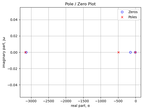

The code below generates a table that lists the values of the pole and zero locations.

table_header = ['Zeros, Hz', 'Poles, Hz']
num_table_rows = max(len(sys_zeros),len(sys_poles))
table_row = []

for i in range(num_table_rows):
    if i < len(sys_zeros):
        z = '{:.2f}'.format(sys_zeros[i]/(2*np.pi))
    else:
        z = ''
    if i < len(sys_poles):
        p = '{:.2f}'.format(sys_poles[i]/(2*np.pi))
    else:
        p = ''
    table_row.append([z,p])

print(tabulate(table_row, headers=table_header,colalign = ('left','left'),tablefmt="simple"))

Zeros, Hz    Poles, Hz
-----------  -----------
-3142.62     -3161.52
-151.29      -491.22
-6.59        -6.6

39.3.6.5 Reactive Branch 3b Frequency Response

The amplitude and phase of the reactive branch is plotted below.

# setup
x_axis = np.logspace(1, 5, 2000, endpoint=False)*2*np.pi
color_list = ['tab:blue','tab:red','tab:green','tab:orange','k']
#gain_setting = np.array([1,25,50,75,99])/100
#p1_value = 100e3

#tf_num_coef_list = []
#tf_denom_coef_list = []

#clean_path1_mag = np.zeros((len(gain_setting),len(x_axis)))

#color_list = ['tab:blue','tab:red','tab:green','tab:orange','k']

# plot
fig, ax1 = plt.subplots()
ax1.set_ylabel('magnitude, dB')
ax1.set_xlabel('frequency, Hz')

# instantiate a second y-axes that shares the same x-axis
ax2 = ax1.twinx()
color = 'k'

ax2.set_ylabel('phase, deg',color=color)
ax2.tick_params(axis='y', labelcolor=color)


NE = NE_sym.subs(element_values)
U = solve(NE,X)
H = U[v2]/U[v1]
num, denom = fraction(H) #returns numerator and denominator

# convert symbolic to NumPy polynomial
a = np.array(Poly(num, s).all_coeffs(), dtype=float)
b = np.array(Poly(denom, s).all_coeffs(), dtype=float)

#x = np.logspace(1, 5, 2000, endpoint=False)*2*np.pi
w, mag, phase = signal.bode((a, b), w=x_axis) # returns: rad/s, mag in dB, phase in deg
#clean_path1_mag[i] = mag

# plot the results
i=0
ax1.semilogx(w/(2*np.pi), mag,'-k',label='mag')    # magnitude plot
ax2.semilogx(w/(2*np.pi), phase,':k',label='phase')  # phase plot

# highlight the guitar audio band, 80 to 8kHz
plt.axvspan(80, 8e3, color='y', alpha=0.3) 

ax1.set_ylim((0,40))

# position legends
ax1.legend(loc='upper left')
ax2.legend(loc='upper right')

ax1.grid()
plt.title('Magnitude and phase response')

plt.show()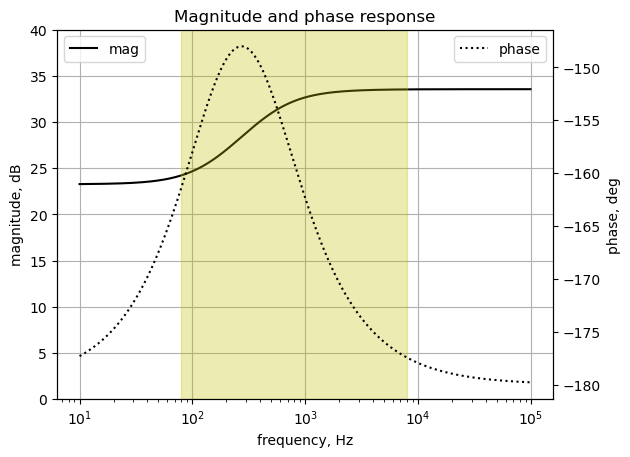

As shown in the amplitude response, there is a lot of gain in this path since \(R_{20}\) is relatively large compared to the impedance of the other components connected to the non-inverting input of \(U_{2A}\). One thing to keep in mind is that the effect of \(C_{13}\) is not included in the plot above. The zero created at 500 Hz by \(C_{13}\) creates a dominating low pass response, which makes me wonder how much do the components \(C_{11}\) and \(C_{12}\) contribute to the overall tone created by the pedal.

39.3.7 Reactive Branch 4

Reactive branch 4 is the circuit path following the diodes, \(D_2\) and \(D_3\) and shown in Figure 37.21. The diodes have been commented out in this analysis and \(V_1\) has been turned off and \(V_2\) is set to a value of 1. The source \(V_2\) represents the signal after the diode shaping. In Figure 39.3 the components from reactive paths 3 and 4 are connected at the non-inverting terminals of \(U_{2A}\). This makes the netlist rather long and the number of equations makes a symbolic solution impracticable. Notice that \(C_{13}\) is not included in the netlist, which is noted below.

Reactive_branch_3_4_net_list = '''
* Reactive_branch_3&4.asc
V1 1 0 0
V2 6 0 1
R5 1 3 5.1e3
R8 3 0 1.5e3
C4 1 3 68e-9
C6 3 4 390e-9
R9 4 0 1e3
Rp1b2 3 5 50e3
Rp1a2 5 0 50e3
R13 8 7 1e3
C11 9 11 2.2e-9
R15 11 5 22e3
R17 10 5 27e3
R18 12 5 12e3
C12 10 12 27e-9
R16 10 9 47e3
*R20 2 10 100e3
R20 2 10 393e3
*C13 2 10 820e-12
O2a 10 0 2
*D2 0 8 1N34A
*D3 8 0 1N34A
C9 6 7 1e-6
C10 9 8 1e-6
'''

The following code takes the netlist and builds and displays the MNA equations.

report, network_df, i_unk_df, A, X, Z = SymMNA.smna(Reactive_branch_3_4_net_list)

# Put matrices into SymPy 
X = Matrix(X)
Z = Matrix(Z)

NE_sym = Eq(A*X,Z)

# display the equations
temp = ''
for i in range(shape(NE_sym.lhs)[0]):
    temp += '${:s} = {:s}$<br>'.format(latex(NE_sym.rhs[i]),latex(NE_sym.lhs[i]))
Markdown(temp)

\(0 = I_{V1} + v_{1} \left(C_{4} s + \frac{1}{R_{5}}\right) + v_{3} \left(- C_{4} s - \frac{1}{R_{5}}\right)\)
\(0 = I_{O2a} - \frac{v_{10}}{R_{20}} + \frac{v_{2}}{R_{20}}\)
\(0 = - C_{6} s v_{4} + v_{1} \left(- C_{4} s - \frac{1}{R_{5}}\right) + v_{3} \left(C_{4} s + C_{6} s + \frac{1}{Rp1b2} + \frac{1}{R_{8}} + \frac{1}{R_{5}}\right) - \frac{v_{5}}{Rp1b2}\)
\(0 = - C_{6} s v_{3} + v_{4} \left(C_{6} s + \frac{1}{R_{9}}\right)\)
\(0 = v_{5} \cdot \left(\frac{1}{Rp1b2} + \frac{1}{Rp1a2} + \frac{1}{R_{18}} + \frac{1}{R_{17}} + \frac{1}{R_{15}}\right) - \frac{v_{3}}{Rp1b2} - \frac{v_{12}}{R_{18}} - \frac{v_{10}}{R_{17}} - \frac{v_{11}}{R_{15}}\)
\(0 = C_{9} s v_{6} - C_{9} s v_{7} + I_{V2}\)
\(0 = - C_{9} s v_{6} + v_{7} \left(C_{9} s + \frac{1}{R_{13}}\right) - \frac{v_{8}}{R_{13}}\)
\(0 = - C_{10} s v_{9} + v_{8} \left(C_{10} s + \frac{1}{R_{13}}\right) - \frac{v_{7}}{R_{13}}\)
\(0 = - C_{10} s v_{8} - C_{11} s v_{11} + v_{9} \left(C_{10} s + C_{11} s + \frac{1}{R_{16}}\right) - \frac{v_{10}}{R_{16}}\)
\(0 = - C_{12} s v_{12} + v_{10} \left(C_{12} s + \frac{1}{R_{20}} + \frac{1}{R_{17}} + \frac{1}{R_{16}}\right) - \frac{v_{2}}{R_{20}} - \frac{v_{5}}{R_{17}} - \frac{v_{9}}{R_{16}}\)
\(0 = - C_{11} s v_{9} + v_{11} \left(C_{11} s + \frac{1}{R_{15}}\right) - \frac{v_{5}}{R_{15}}\)
\(0 = - C_{12} s v_{10} + v_{12} \left(C_{12} s + \frac{1}{R_{18}}\right) - \frac{v_{5}}{R_{18}}\)
\(V_{1} = v_{1}\)
\(V_{2} = v_{6}\)
\(0 = v_{10}\)

Turn the free symbols into SymPy variables and load the element values.

var(str(NE_sym.free_symbols).replace('{','').replace('}',''))
element_values = SymMNA.get_part_values(network_df)

39.3.7.1 Numerical Solution for P1 at 50%

Substitute the component values into the network equations and display the numerical equations.

equ_N = NE_sym.subs(element_values)

temp = ''
for i in range(shape(equ_N.lhs)[0]):
    temp += '<p>${:s} = {:s}$</p>'.format(latex(equ_N.rhs[i]),
        latex(round_expr(equ_N.lhs[i],7)))

Markdown(temp)

\(0 = I_{V1} + v_{1} \cdot \left(1.0 \cdot 10^{-7} s + 0.0001961\right) + v_{3} \left(- 1.0 \cdot 10^{-7} s - 0.0001961\right)\)

\(0 = I_{O2a} - 2.5 \cdot 10^{-6} v_{10} + 2.5 \cdot 10^{-6} v_{2}\)

\(0 = - 4.0 \cdot 10^{-7} s v_{4} + v_{1} \left(- 1.0 \cdot 10^{-7} s - 0.0001961\right) + v_{3} \cdot \left(5.0 \cdot 10^{-7} s + 0.0008827\right) - 2.0 \cdot 10^{-5} v_{5}\)

\(0 = - 4.0 \cdot 10^{-7} s v_{3} + v_{4} \cdot \left(4.0 \cdot 10^{-7} s + 0.001\right)\)

\(0 = - 3.7 \cdot 10^{-5} v_{10} - 4.55 \cdot 10^{-5} v_{11} - 8.33 \cdot 10^{-5} v_{12} - 2.0 \cdot 10^{-5} v_{3} + 0.0002058 v_{5}\)

\(0 = I_{V2} + 1.0 \cdot 10^{-6} s v_{6} - 1.0 \cdot 10^{-6} s v_{7}\)

\(0 = - 1.0 \cdot 10^{-6} s v_{6} + v_{7} \cdot \left(1.0 \cdot 10^{-6} s + 0.001\right) - 0.001 v_{8}\)

\(0 = - 1.0 \cdot 10^{-6} s v_{9} - 0.001 v_{7} + v_{8} \cdot \left(1.0 \cdot 10^{-6} s + 0.001\right)\)

\(0 = - 1.0 \cdot 10^{-6} s v_{8} - 2.13 \cdot 10^{-5} v_{10} + v_{9} \cdot \left(1.0 \cdot 10^{-6} s + 2.13 \cdot 10^{-5}\right)\)

\(0 = 6.09 \cdot 10^{-5} v_{10} - 2.5 \cdot 10^{-6} v_{2} - 3.7 \cdot 10^{-5} v_{5} - 2.13 \cdot 10^{-5} v_{9}\)

\(0 = 4.55 \cdot 10^{-5} v_{11} - 4.55 \cdot 10^{-5} v_{5}\)

\(0 = 8.33 \cdot 10^{-5} v_{12} - 8.33 \cdot 10^{-5} v_{5}\)

\(0 = v_{1}\)

\(1.0 = v_{6}\)

\(0 = v_{10}\)

SymPy can solve for unknown node voltages and the unknown currents from the independent voltage source, \(V_2\), and the Op Amp’s output terminal. The unknown currents, \(I_{V1}\) and \(I_{O1}\), are not displayed. The node voltages are:

U = solve(equ_N,X)

temp = ''
for i in U.keys():
    if str(i)[0] == 'v': # only display the node voltages
        temp += '<p>${:s} = {:s}$</p>'.format(latex(i),latex(U[i]))

Markdown(temp)

\(v_{1} = 0.0\)

\(v_{2} = \frac{- 1.96394441888298 \cdot 10^{71} s^{5} - 7.60825164075479 \cdot 10^{75} s^{4} - 5.90607987153688 \cdot 10^{79} s^{3} - 1.18301509344067 \cdot 10^{83} s^{2} - 6.89566385064667 \cdot 10^{85} s}{1.10336500111661 \cdot 10^{70} s^{5} + 5.26456182674577 \cdot 10^{74} s^{4} + 6.46095251106143 \cdot 10^{78} s^{3} + 1.43698004458909 \cdot 10^{82} s^{2} + 9.04296553120415 \cdot 10^{84} s + 3.50924368989652 \cdot 10^{86}}\)

\(v_{3} = \frac{2.9615625 \cdot 10^{56} s^{4} + 1.6734375 \cdot 10^{60} s^{3} + 2.34375 \cdot 10^{63} s^{2}}{4.81802717154256 \cdot 10^{54} s^{5} + 2.29885866434566 \cdot 10^{59} s^{4} + 2.82128259649683 \cdot 10^{63} s^{3} + 6.27481286137239 \cdot 10^{66} s^{2} + 3.94876161529248 \cdot 10^{69} s + 1.53236974458815 \cdot 10^{71}}\)

\(v_{4} = \frac{2.9615625 \cdot 10^{56} s^{4} + 9.14062499999999 \cdot 10^{59} s^{3}}{4.81802717154256 \cdot 10^{54} s^{5} + 2.29885866434566 \cdot 10^{59} s^{4} + 2.82128259649683 \cdot 10^{63} s^{3} + 6.27481286137239 \cdot 10^{66} s^{2} + 3.94876161529248 \cdot 10^{69} s + 1.53236974458815 \cdot 10^{71}}\)

\(v_{5} = \frac{1.00693125 \cdot 10^{54} s^{5} + 3.35690238970588 \cdot 10^{58} s^{4} + 1.275328125 \cdot 10^{62} s^{3} + 1.0344669117647 \cdot 10^{65} s^{2}}{4.81802717154256 \cdot 10^{54} s^{5} + 2.29885866434566 \cdot 10^{59} s^{4} + 2.82128259649683 \cdot 10^{63} s^{3} + 6.27481286137239 \cdot 10^{66} s^{2} + 3.94876161529248 \cdot 10^{69} s + 1.53236974458815 \cdot 10^{71}}\)

\(v_{6} = 1.0\)

\(v_{7} = \frac{4.81802717154256 \cdot 10^{54} s^{5} + 2.29627373138023 \cdot 10^{59} s^{4} + 2.81149214573178 \cdot 10^{63} s^{3} + 6.20412190793865 \cdot 10^{66} s^{2} + 3.81322450115202 \cdot 10^{69} s + 7.66184872294075 \cdot 10^{70}}{4.81802717154256 \cdot 10^{54} s^{5} + 2.29885866434566 \cdot 10^{59} s^{4} + 2.82128259649683 \cdot 10^{63} s^{3} + 6.27481286137239 \cdot 10^{66} s^{2} + 3.94876161529248 \cdot 10^{69} s + 1.53236974458815 \cdot 10^{71}}\)

\(v_{8} = \frac{4.559533875 \cdot 10^{54} s^{5} + 2.19836922372969 \cdot 10^{59} s^{4} + 2.74080119229803 \cdot 10^{63} s^{3} + 6.06858479379818 \cdot 10^{66} s^{2} + 3.73660601392261 \cdot 10^{69} s + 7.66184872294075 \cdot 10^{70}}{4.81802717154256 \cdot 10^{54} s^{5} + 2.29885866434566 \cdot 10^{59} s^{4} + 2.82128259649683 \cdot 10^{63} s^{3} + 6.27481286137239 \cdot 10^{66} s^{2} + 3.94876161529248 \cdot 10^{69} s + 1.53236974458815 \cdot 10^{71}}\)

\(v_{9} = \frac{4.559533875 \cdot 10^{54} s^{5} + 2.19578429076426 \cdot 10^{59} s^{4} + 2.73101074153298 \cdot 10^{63} s^{3} + 5.99789384036444 \cdot 10^{66} s^{2} + 3.60106889978214 \cdot 10^{69} s}{4.81802717154256 \cdot 10^{54} s^{5} + 2.29885866434566 \cdot 10^{59} s^{4} + 2.82128259649683 \cdot 10^{63} s^{3} + 6.27481286137239 \cdot 10^{66} s^{2} + 3.94876161529248 \cdot 10^{69} s + 1.53236974458815 \cdot 10^{71}}\)

\(v_{10} = 0.0\)

\(v_{11} = \frac{4.559533875 \cdot 10^{54} s^{5} + 1.46177548394608 \cdot 10^{59} s^{4} + 4.04388334558824 \cdot 10^{62} s^{3} + 2.77738425925926 \cdot 10^{65} s^{2}}{4.81802717154256 \cdot 10^{54} s^{5} + 2.29885866434566 \cdot 10^{59} s^{4} + 2.82128259649683 \cdot 10^{63} s^{3} + 6.27481286137239 \cdot 10^{66} s^{2} + 3.94876161529248 \cdot 10^{69} s + 1.53236974458815 \cdot 10^{71}}\)

\(v_{12} = \frac{3.1078125 \cdot 10^{57} s^{4} + 9.40160845588234 \cdot 10^{61} s^{3} + 1.0344669117647 \cdot 10^{65} s^{2}}{4.81802717154256 \cdot 10^{54} s^{5} + 2.29885866434566 \cdot 10^{59} s^{4} + 2.82128259649683 \cdot 10^{63} s^{3} + 6.27481286137239 \cdot 10^{66} s^{2} + 3.94876161529248 \cdot 10^{69} s + 1.53236974458815 \cdot 10^{71}}\)

The network transfer function, \(H(s)=\frac {v_2(s)}{v_1(s)}\), is:

H = (U[v2]/U[v6]).cancel()
Markdown('$H(s)={:s}$'.format(latex(H)))

\(H(s)=\frac{- 1.96394441888298 \cdot 10^{71} s^{5} - 7.60825164075479 \cdot 10^{75} s^{4} - 5.90607987153688 \cdot 10^{79} s^{3} - 1.18301509344067 \cdot 10^{83} s^{2} - 6.89566385064667 \cdot 10^{85} s}{1.10336500111661 \cdot 10^{70} s^{5} + 5.26456182674577 \cdot 10^{74} s^{4} + 6.46095251106143 \cdot 10^{78} s^{3} + 1.43698004458909 \cdot 10^{82} s^{2} + 9.04296553120415 \cdot 10^{84} s + 3.50924368989652 \cdot 10^{86}}\)

The SciPy function, TransferFunction, is used to represent the system as the continuous-time transfer function. The code below extracts the numerator and denominator polynomials from the voltage transfer function. Then coefficients of the terms are used to build a SciPy transfer function object.

H_num, H_denom = fraction(H) #returns numerator and denominator

# convert symbolic to NumPy polynomial
a = np.array(Poly(H_num, s).all_coeffs(), dtype=float)
b = np.array(Poly(H_denom, s).all_coeffs(), dtype=float)

sys_tf = signal.TransferFunction(a,b)

39.3.7.2 Pole Zero Plot

The poles and zeros of the transfer function can easily be obtained with the following code:

sys_zeros = np.roots(sys_tf.num)
sys_poles = np.roots(sys_tf.den)

The poles and zeros of the transfer function are plotted on the complex frequency plane with the following code:

plt.plot(np.real(sys_zeros/(2*np.pi)), np.imag(sys_zeros/(2*np.pi)), 'ob', markerfacecolor='none')
plt.plot(np.real(sys_poles/(2*np.pi)), np.imag(sys_poles/(2*np.pi)), 'xr')
plt.legend(['Zeros', 'Poles'], loc=0)
plt.title('Pole / Zero Plot')
plt.xlabel('real part, \u03B1')
plt.ylabel('imaginary part, j\u03C9')
plt.grid()
plt.show()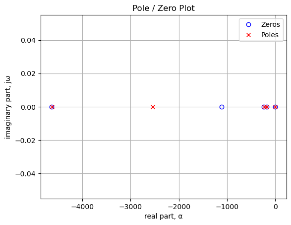

The code below generates a table that lists the values of the pole and zero locations.

table_header = ['Zeros, Hz', 'Poles, Hz']
num_table_rows = max(len(sys_zeros),len(sys_poles))
table_row = []

for i in range(num_table_rows):
    if i < len(sys_zeros):
        z = '{:.2f}'.format(sys_zeros[i]/(2*np.pi))
    else:
        z = ''
    if i < len(sys_poles):
        p = '{:.2f}'.format(sys_poles[i]/(2*np.pi))
    else:
        p = ''
    table_row.append([z,p])

print(tabulate(table_row, headers=table_header,colalign = ('left','left'),tablefmt="simple"))

Zeros, Hz    Poles, Hz
-----------  -----------
-4631.99     -4629.79
-1110.36     -2545.69
-243         -231.62
-180.26      -180.17
0            -6.6

39.3.7.3 Pole/Zero Locus Plot versus P1 value

There are six zeros and six poles. The code below solves the network equations and finds the numerator and denominator roots of the transfer function for various rotation positions of \(P_1\).

p1_value = 100e3
num_roots = []
denom_roots = []
for i in np.linspace(1,99,20)/100:
    element_values[Rp1a2] = p1_value - i*p1_value
    element_values[Rp1b2] = i*p1_value
    
    NE = NE_sym.subs(element_values)
    U = solve(NE,X)
    H = U[v2]/U[v6]
    num, denom = fraction(H) #returns numerator and denominator

    # convert symbolic to NumPy polynomial
    a = np.array(Poly(num, s).all_coeffs(), dtype=float)
    b = np.array(Poly(denom, s).all_coeffs(), dtype=float)    
    sys_tf = signal.TransferFunction(a,b)
    
    num_roots.append(np.roots(sys_tf.num))
    denom_roots.append(np.roots(sys_tf.den))

The range of values taken on by the zeros as \(P_1\) is rotated are printed below.

# put the zeros into an array
z0_locus = np.zeros(len(np.array(num_roots)))
z1_locus = np.zeros(len(np.array(num_roots)))
z2_locus = np.zeros(len(np.array(num_roots)))
z3_locus = np.zeros(len(np.array(num_roots)))
z4_locus = np.zeros(len(np.array(num_roots)))

for i in range(len(np.array(num_roots))):
    z0_locus[i] = -np.array(num_roots)[i][0]    
    z1_locus[i] = -np.array(num_roots)[i][1]        
    z2_locus[i] = -np.array(num_roots)[i][2]    
    z3_locus[i] = -np.array(num_roots)[i][3]  
    z4_locus[i] = -np.array(num_roots)[i][4]    

print(f'z0 range as a function of P1: {z0_locus.min()/(2*np.pi)/1e3:.3f} to {z0_locus.max()/(2*np.pi)/1e3:.3f} kHz')
print(f'z1 range as a function of P1: {z1_locus.min()/(2*np.pi)/1e3:.3f} to {z1_locus.max()/(2*np.pi)/1e3:.3f} kHz')
print(f'z2 range as a function of P1: {z2_locus.min()/(2*np.pi)/1e3:.3f} to {z2_locus.max()/(2*np.pi)/1e3:.3f} kHz')
print(f'z3 range as a function of P1: {z3_locus.min()/(2*np.pi)/1e3:.3f} to {z3_locus.max()/(2*np.pi)/1e3:.3f} kHz')
print(f'z4 range as a function of P1: {z4_locus.min()/(2*np.pi)/1e3:.3f} to {z4_locus.max()/(2*np.pi)/1e3:.3f} kHz')

z0 range as a function of P1: 4.611 to 5.652 kHz
z1 range as a function of P1: 1.111 to 2.529 kHz
z2 range as a function of P1: 0.243 to 0.467 kHz
z3 range as a function of P1: 0.179 to 0.181 kHz
z4 range as a function of P1: -0.000 to -0.000 kHz

The plot provides a visual indication of how the zeros change in frequency as a function of the rotational position of \(P_1\).

plt.plot(np.linspace(1,99,len(np.array(num_roots))),z0_locus/(2*np.pi)/1e3,'x-', markerfacecolor='none',label='z_0')
plt.plot(np.linspace(1,99,len(np.array(num_roots))),z1_locus/(2*np.pi)/1e3,'x-', markerfacecolor='none',label='z_1')
plt.plot(np.linspace(1,99,len(np.array(num_roots))),z2_locus/(2*np.pi)/1e3,'x-', markerfacecolor='none',label='z_2')
plt.plot(np.linspace(1,99,len(np.array(num_roots))),z3_locus/(2*np.pi)/1e3,'x-', markerfacecolor='none',label='z_3')

plt.ylim((0,6))
plt.legend(loc='upper left')
plt.title('Gain control pole & zero frequency plot vs gain rotation %')
plt.xlabel('Gain rotation percentage')
plt.ylabel('pole and zero frequency, kHz')
plt.grid()

plt.show()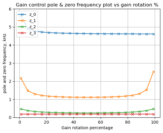

As shown above, the zeros are relatively constant versus \(P_1\) for most of the rotational range.

The range of values for each of the poles as function of \(P_1\) are printed below.

# put the poles into an array
p0_locus = np.zeros(len(np.array(denom_roots)))
p1_locus = np.zeros(len(np.array(denom_roots)))
p2_locus = np.zeros(len(np.array(denom_roots)))
p3_locus = np.zeros(len(np.array(denom_roots)))
p4_locus = np.zeros(len(np.array(denom_roots)))

for i in range(len(np.array(denom_roots))):
    p0_locus[i] = -np.array(denom_roots)[i][0]    
    p1_locus[i] = -np.array(denom_roots)[i][1]       
    p2_locus[i] = -np.array(denom_roots)[i][2]      
    p3_locus[i] = -np.array(denom_roots)[i][3]      
    p4_locus[i] = -np.array(denom_roots)[i][4]      

print(f'p0 range as a function of P1: {p0_locus.min()/(2*np.pi)/1e3:.3f} to {p0_locus.max()/(2*np.pi)/1e3:.3f} kHz')
print(f'p1 range as a function of P1: {p1_locus.min()/(2*np.pi)/1e3:.3f} to {p1_locus.max()/(2*np.pi)/1e3:.3f} kHz')
print(f'p2 range as a function of P1: {p2_locus.min()/(2*np.pi)/1e3:.3f} to {p2_locus.max()/(2*np.pi)/1e3:.3f} kHz')
print(f'p3 range as a function of P1: {p3_locus.min()/(2*np.pi)/1e3:.3f} to {p3_locus.max()/(2*np.pi)/1e3:.3f} kHz')
print(f'p4 range as a function of P1: {p4_locus.min()/(2*np.pi)/1e3:.3f} to {p4_locus.max()/(2*np.pi)/1e3:.3f} kHz')

p0 range as a function of P1: 4.611 to 5.043 kHz
p1 range as a function of P1: 2.546 to 3.046 kHz
p2 range as a function of P1: 0.232 to 0.455 kHz
p3 range as a function of P1: 0.179 to 0.181 kHz
p4 range as a function of P1: 0.007 to 0.007 kHz

The plot provides a visual indication of how the poles change in frequency as a function of the rotational position of \(P_1\).

plt.plot(np.linspace(1,99,len(np.array(denom_roots))),p0_locus/(2*np.pi)/1e3,'x-', markerfacecolor='none',label='p_0')
plt.plot(np.linspace(1,99,len(np.array(denom_roots))),p1_locus/(2*np.pi)/1e3,'x-', markerfacecolor='none',label='p_1')
plt.plot(np.linspace(1,99,len(np.array(denom_roots))),p2_locus/(2*np.pi)/1e3,'x-', markerfacecolor='none',label='p_2')
plt.plot(np.linspace(1,99,len(np.array(denom_roots))),p3_locus/(2*np.pi)/1e3,'x-', markerfacecolor='none',label='p_3')

plt.ylim((0,6))
plt.legend(loc='upper left')
plt.title('Gain control pole & zero frequency plot vs gain rotation %')
plt.xlabel('Gain rotation percentage')
plt.ylabel('pole and zero frequency, kHz')
plt.grid()

plt.show()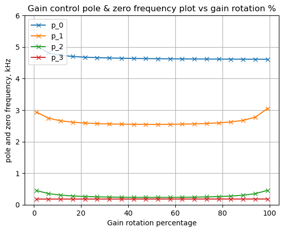

As shown above, the poles are relatively constant versus \(P_1\) for most of the rotational range.

39.3.7.4 Reactive Branch 4 Frequency Response

The frequency response of reactive branch 4 is plotted below. The gain setting is a percent of full scale.

# setup
x_axis = np.logspace(1, 5, 2000, endpoint=False)*2*np.pi
color_list = ['tab:blue','tab:red','tab:green','tab:orange','k']
gain_setting = np.array([1,25,50,75,99])/100
p1_value = 100e3

#tf_num_coef_list = []
#tf_denom_coef_list = []

#clean_path1_mag = np.zeros((len(gain_setting),len(x_axis)))

#color_list = ['tab:blue','tab:red','tab:green','tab:orange','k']

# plot
fig, ax1 = plt.subplots()
ax1.set_ylabel('magnitude, dB')
ax1.set_xlabel('frequency, Hz')

# instantiate a second y-axes that shares the same x-axis
ax2 = ax1.twinx()
color = 'k'

ax2.set_ylabel('phase, deg',color=color)
ax2.tick_params(axis='y', labelcolor=color)

for i in range(len(gain_setting)):
    element_values[Rp1a2] = p1_value - gain_setting[i]*p1_value
    element_values[Rp1b2] = gain_setting[i]*p1_value
    
    #element_values[Rp1a2] = p1_value - gain_setting[i]*p1_value
    #element_values[Rp1b2] = gain_setting[i]*p1_value
    
    NE = NE_sym.subs(element_values)
    U = solve(NE,X)
    H = U[v2]/U[v6]
    num, denom = fraction(H) #returns numerator and denominator

    # convert symbolic to NumPy polynomial
    a = np.array(Poly(num, s).all_coeffs(), dtype=float)
    b = np.array(Poly(denom, s).all_coeffs(), dtype=float)
    #tf_num_coef_list.append(a)
    #tf_denom_coef_list.append(b)
    
    #x = np.logspace(1, 5, 2000, endpoint=False)*2*np.pi
    w, mag, phase = signal.bode((a, b), w=x_axis) # returns: rad/s, mag in dB, phase in deg
    #clean_path1_mag[i] = mag
    
    # plot the results.  
    ax1.semilogx(w/(2*np.pi), mag,'-',color=color_list[i],label='mag: {:.0f}%'.format(gain_setting[i]*100))    # magnitude plot
    ax2.semilogx(w/(2*np.pi), phase,':',color=color_list[i],label='phase: {:.0f}%'.format(gain_setting[i]*100))  # phase plot

# highlight the guitar audio band, 80 to 8kHz
plt.axvspan(80, 8e3, color='y', alpha=0.3) 

#ax1.set_ylim((0,15))

# position legends outside the graph
ax1.legend(bbox_to_anchor=(1.6,1)) # magnitude legend position: relative (horizontal position, vertical position) 
ax2.legend(bbox_to_anchor=(1.6,0.5)) # phase legend position:

#ax1.legend(loc='lower left')
#ax2.legend(loc='lower right')
ax1.grid()
plt.title('Magnitude and phase response')
#plt.savefig('reactive_path_4_bode.png')
plt.show()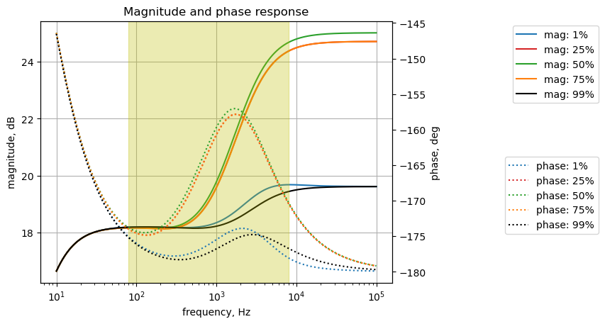

The plot above shows that influence of the rotation of \(P_1\) has a large effect on the amplitude response at \(P_1\) rotational positions of 50 and 75%. However when \(C_{13}\) is included in the analysis, the zero created at about 500 Hz greatly influences the response along this path as shown in the plot below.

Reactive path 4 with \(C_{13}\) included in the netlist.

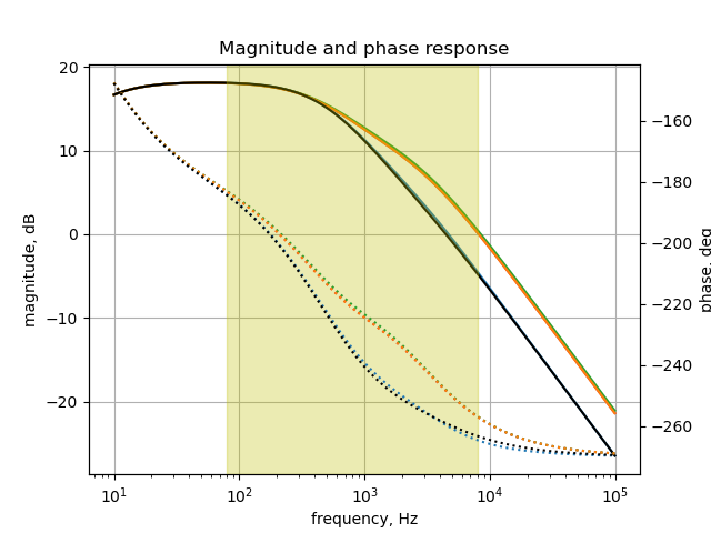
39.4 Summary

The Klon Centaur is a famous, highly sought-after and legendary guitar pedal. The pedal was adopted by some notable players (Jeff Beck, Mark Tremonti, John Mayer, Andy Summers, Peter Frampton, Jason Isbell, James Hetfield, Joe Perry, Britt Daniel, David Grissom, Adam Hann, Joe Bonamassa). The limited initial production and long wait times led to its rarity and high demand.

Working on this series of JupyterLab pages has given me the opportunity to to learn a few things about electric guitars and pedals. If I were to continue farther down this path, the next step would be to build some breadboard circuits and verify my analysis by comparing calculated with measured results.

Here are a few of my observations:

• Clean path 1 not contributing much and signals on this path appear to be covered by the clean path 2 and the diode path.
• Reactive branches 3 and 4 are unusual filters
  • Branch 3 provides 20 dB of emphasis across the guitar audio band
  • Branch 4 provides 3 to 4 dB of emphasis across the guitar audio band
    
  • Both seem superfluous and appear to be dominated by \(R_{20}\) and \(C_{13}\)

Basso, Christophe. 2016. “Introduction to Fast Analytical Techniques: Application to Small-Signal Modeling.” 2016. https://www.powersimtof.com/Downloads/PPTs/Chris%20Basso%20APEC%20seminar%202016.pdf.

Middlebrook, R. D., V. Vorperian, and J. Lindal. 1998. “The n Extra Element Theorem.” IEEE Transactions on Circuits and Systems I: Fundamental Theory and Applications 45 (9): 919–35. https://doi.org/10.1109/81.721258.