from sympy import *
import numpy as np
from tabulate import tabulate
from scipy import signal
import matplotlib.pyplot as plt
import pandas as pd
import SymMNA
from IPython.display import display, Markdown, Math, Latex
init_printing()20 Super Node

A question posted on Electronics Stackexchange by Malek (2020) asked:
I have a circuit that I would like to convert into a conductance matrix for the node analysis by inspection method. I have, however, run into a problem. I have this 36V ideal voltage source with no resistance on its branch, which means that I cannot convert it into a current source with the Norton/Thenevin equivalent circuit theorem (or can I?). I have thought of making the third node connected to the voltage source dependent on the first node connected to the voltage source, i.e. v1 = v1 + 36. I have tried this method, but I do not get the correct values. Am I messing up? Is there no way to handle ideal voltage sources with the node analysis by inspection method?
The MNA solution provided below can work directly with the circuit netlist and the concept of a super node is not required.
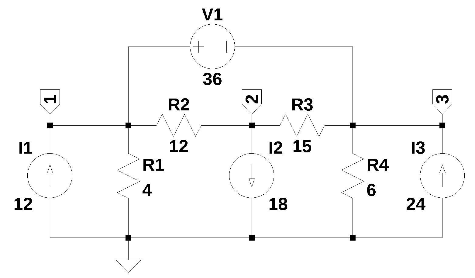
The net list for Figure 31.1 was generated by LTSpice and show below:
V1 1 3 36
I1 0 1 12
I2 2 0 18
I3 0 3 24
R1 1 0 4
R4 3 0 6
R2 2 1 12
R3 3 2 15
The following Python modules are used in this notebook.
20.1 Load the net list
The netlist for the circuit is pasted into the code cell below. In Python a triple-quoted string includes whitespace, tabs and newlines. The newlines characters are needed to mark the end of each SPICE statement in the netlist.
net_list = '''
V1 1 3 36
I1 0 1 12
I2 2 0 18
I3 0 3 24
R1 1 0 4
R4 3 0 6
R2 2 1 12
R3 3 2 15
'''
20.2 Call the symbolic modified nodal analysis function
report, network_df, i_unk_df, A, X, Z = SymMNA.smna(net_list)The network equations for the circuit can be obtained from the A, X and Z values returned from the smna function. The A, X and Z are formuloated into equations and displayed below. Markdown is an IPython function and latex is a SymPy printing function.
# Put matrices into SymPy
X = Matrix(X)
Z = Matrix(Z)

NE_sym = Eq(A*X,Z)

# turn the free symbols into SymPy variables.
var(str(NE_sym.free_symbols).replace('{','').replace('}',''))

# construct a dictionary of element values
element_values = SymMNA.get_part_values(network_df)

temp = ''
for i in range(len(X)):
    temp += '${:s}$<br>'.format(latex(Eq((A*X)[i:i+1][0],Z[i])))

Markdown(temp)
\(I_{V1} + v_{1} \cdot \left(\frac{1}{R_{2}} + \frac{1}{R_{1}}\right) - \frac{v_{2}}{R_{2}} = I_{1}\)
\(v_{2} \cdot \left(\frac{1}{R_{3}} + \frac{1}{R_{2}}\right) - \frac{v_{3}}{R_{3}} - \frac{v_{1}}{R_{2}} = - I_{2}\)
\(- I_{V1} + v_{3} \cdot \left(\frac{1}{R_{4}} + \frac{1}{R_{3}}\right) - \frac{v_{2}}{R_{3}} = I_{3}\)
\(v_{1} - v_{3} = V_{1}\)
20.3 Symbolic solution
The newtork equations can be solved symbolically.
U_sym = solve(NE_sym,X)

# display the symbolic solution
temp = ''
for i in U_sym.keys():
    temp += '${:s} = {:s}$<br>'.format(latex(i),latex(U_sym[i]))

Markdown(temp)
\(v_{1} = \frac{I_{1} R_{1} R_{4} - I_{2} R_{1} R_{4} + I_{3} R_{1} R_{4} + R_{1} V_{1}}{R_{1} + R_{4}}\)
\(v_{2} = \frac{I_{1} R_{1} R_{2} R_{4} + I_{1} R_{1} R_{3} R_{4} - I_{2} R_{1} R_{2} R_{3} - I_{2} R_{1} R_{2} R_{4} - I_{2} R_{1} R_{3} R_{4} - I_{2} R_{2} R_{3} R_{4} + I_{3} R_{1} R_{2} R_{4} + I_{3} R_{1} R_{3} R_{4} + R_{1} R_{3} V_{1} - R_{2} R_{4} V_{1}}{R_{1} R_{2} + R_{1} R_{3} + R_{2} R_{4} + R_{3} R_{4}}\)
\(v_{3} = \frac{I_{1} R_{1} R_{4} - I_{2} R_{1} R_{4} + I_{3} R_{1} R_{4} - R_{4} V_{1}}{R_{1} + R_{4}}\)
\(I_{V1} = \frac{I_{1} R_{1} R_{2} + I_{1} R_{1} R_{3} - I_{2} R_{1} R_{3} + I_{2} R_{2} R_{4} - I_{3} R_{2} R_{4} - I_{3} R_{3} R_{4} - R_{1} V_{1} - R_{2} V_{1} - R_{3} V_{1} - R_{4} V_{1}}{R_{1} R_{2} + R_{1} R_{3} + R_{2} R_{4} + R_{3} R_{4}}\)
20.4 Numerical solution
NE = NE_sym.subs(element_values)

# display the equations with numerical values
temp = ''
for i in range(shape(NE.lhs)[0]):
    temp += '${:s} = {:s}$<br>'.format(latex(NE.rhs[i]),latex(NE.lhs[i]))

Markdown(temp)
\(12.0 = I_{V1} + 0.333333333333333 v_{1} - 0.0833333333333333 v_{2}\)
\(-18.0 = - 0.0833333333333333 v_{1} + 0.15 v_{2} - 0.0666666666666667 v_{3}\)
\(24.0 = - I_{V1} - 0.0666666666666667 v_{2} + 0.233333333333333 v_{3}\)
\(36.0 = v_{1} - v_{3}\)
Use SymPy to solve the equations.
U = solve(NE,X)Display the numerical solution. Six significant digits are displayed so that results can be compared to LTSpice.
table_header = ['unknown', 'mag']
table_row = []

for name, value in U.items():
    table_row.append([str(name),float(value)])

print(tabulate(table_row, headers=table_header,colalign = ('left','decimal'),tablefmt="simple",floatfmt=('5s','.6f')))
unknown mag
--------- ----------
v1 57.600000
v2 -78.400000
v3 21.600000
I_V1 -13.733333The node voltages and current through the sources are solved for. The Sympy generated solution matches the LTSpice results:
       --- Operating Point ---

V(1):    57.6    voltage
V(3):    21.6    voltage
V(2):    -78.4   voltage
I(I1):   12  device_current
I(I2):   18  device_current
I(I3):   24  device_current
I(R1):   14.4    device_current
I(R4):   3.6     device_current
I(R2):   -11.3333    device_current
I(R3):   6.66667     device_current
I(V1):   -13.7333    device_current
The results from LTSpice agree with the SymPy results.
20.5 Summary
The chapter addresses a common challenge in nodal analysis: dealing with voltage sources connected between two non-reference nodes. In traditional nodeal analysis, this requires a “Super Node” approach. However, the chapter demonstrates that by using MNA and Python, these circuits can be solved directly without the need for the Super Node concept.