8  Transient Analysis

Transient analysis in electrical circuit analysis is the study of a circuit’s behavior during the time it transitions from one steady-state condition to another, typically following a sudden change, such as the opening or closing of a switch or an abrupt change in the input signal. This period, known as the transient period, is characterized by time-varying voltages and currents, especially in circuits containing energy-storage elements like capacitors and inductors, whose voltage and current, respectively, cannot change instantaneously.

While steady-state analysis focuses on how a circuit behaves after it has “settled” over a long period, transient analysis examines the volatile interval immediately following a change in the circuit’s topology or excitation. This behavior is governed by the physics of energy storage. In transient analysis, the unit step function, denoted as \(u(t)\), serves as the mathematical model for a switch. It is a function that represents an instantaneous transition from an “off” state to an “on” state at a \(t=0\).

In the frequency, the Laplace transform of the unit step is \(1/s\). This makes it easy to solve differential equations for circuits because it converts a complex “switching” event into a simple algebraic term. Engineers use the Step Response (how a system reacts to a unit step input) to determine critical performance metrics like rise time, overshoot and settling time. If you know how a circuit handles a step function, you can often predict how it will handle any other type of input.

Two example circuits are presented for analysis. They are both LC low pass filters with resistive terminations. The filters have been designed to intentionally include ripple in the pass band and overshoot in the transient response in order to make the plots look a bit more interesting.

Load the following Python modules.

from sympy import *
import numpy as np
from tabulate import tabulate
import pandas as pd
from scipy import signal
import matplotlib.pyplot as plt
import SymMNA
from IPython.display import display, Markdown, Math, Latex
init_printing()

8.1 Circuit Example 1

Figure 8.1: Schematic for circuit example 1.

The circuit in Figure 8.1 is a Chebyshev low pass filter, with a 1 MHz cut off frequency, \(50\Omega\) termination and 3 dB of ripple in the pass band. Three dB of ripple in the pass band was designed in so that the transient response would have some ringing. The filter design tool from Marki Microwave (2025) was used to design the filter.

The netlist generated by LTSpice is pasted into the cell below and some edits were made to remove the inductor series resistance and the independent source, V1, is set to a value of one.

net_list = '''
V1 1 0 1
R1 3 1 50
R2 2 0 50
C1 3 0 10.66e-9
L1 3 2 5.664e-6
C2 2 0 10.66e-9
'''

Generate and display the network equations.

report, network_df, df2, A, X, Z = SymMNA.smna(net_list)

# Put matricies into SymPy 
X = Matrix(X)
Z = Matrix(Z)

NE_sym = Eq(A*X,Z)

# turn the free symbols into SymPy variables
var(str(NE_sym.free_symbols).replace('{','').replace('}',''))

# built a dictionary of element values.
element_values = SymMNA.get_part_values(network_df)

# generate markdown text to display the network equations.
temp = ''
for i in range(len(X)):
    temp += '${:s}$<br>'.format(latex(Eq((A*X)[i:i+1][0],Z[i])))

Markdown(temp)

\(I_{V1} + \frac{v_{1}}{R_{1}} - \frac{v_{3}}{R_{1}} = 0\)
\(- I_{L1} + v_{2} \left(C_{2} s + \frac{1}{R_{2}}\right) = 0\)
\(I_{L1} + v_{3} \left(C_{1} s + \frac{1}{R_{1}}\right) - \frac{v_{1}}{R_{1}} = 0\)
\(v_{1} = V_{1}\)
\(- I_{L1} L_{1} s - v_{2} + v_{3} = 0\)

As shown above MNA generated many equations and these would be difficult to solve by hand. The equations are displade in matrix notation below.

Since the circuit is not too large, a symbolic solution can be easily obtained and displayed.

U_sym = solve(NE_sym,X)

temp = ''
for i in U_sym.keys():
    temp += '${:s} = {:s}$<br>'.format(latex(i),latex(U_sym[i]))

Markdown(temp)

\(v_{1} = V_{1}\)
\(v_{2} = \frac{R_{2} V_{1}}{C_{1} C_{2} L_{1} R_{1} R_{2} s^{3} + C_{1} L_{1} R_{1} s^{2} + C_{1} R_{1} R_{2} s + C_{2} L_{1} R_{2} s^{2} + C_{2} R_{1} R_{2} s + L_{1} s + R_{1} + R_{2}}\)
\(v_{3} = \frac{C_{2} L_{1} R_{2} V_{1} s^{2} + L_{1} V_{1} s + R_{2} V_{1}}{C_{1} C_{2} L_{1} R_{1} R_{2} s^{3} + C_{1} L_{1} R_{1} s^{2} + C_{1} R_{1} R_{2} s + C_{2} L_{1} R_{2} s^{2} + C_{2} R_{1} R_{2} s + L_{1} s + R_{1} + R_{2}}\)
\(I_{V1} = \frac{- C_{1} C_{2} L_{1} R_{2} V_{1} s^{3} - C_{1} L_{1} V_{1} s^{2} - C_{1} R_{2} V_{1} s - C_{2} R_{2} V_{1} s - V_{1}}{C_{1} C_{2} L_{1} R_{1} R_{2} s^{3} + C_{1} L_{1} R_{1} s^{2} + C_{1} R_{1} R_{2} s + C_{2} L_{1} R_{2} s^{2} + C_{2} R_{1} R_{2} s + L_{1} s + R_{1} + R_{2}}\)
\(I_{L1} = \frac{C_{2} R_{2} V_{1} s + V_{1}}{C_{1} C_{2} L_{1} R_{1} R_{2} s^{3} + C_{1} L_{1} R_{1} s^{2} + C_{1} R_{1} R_{2} s + C_{2} L_{1} R_{2} s^{2} + C_{2} R_{1} R_{2} s + L_{1} s + R_{1} + R_{2}}\)

After substituting the numeric component values for the elements, a numerical solution for the note voltages can be obtained.

NE = NE_sym.subs(element_values)
U = solve(NE,X)

The transfer function \(H(s)=\frac {v_2(s)}{v_1(s)}\) is obtained below and plotted.

H = U[v2]/U[v1]

num, denom = fraction(H) #returns numerator and denominator

# convert symbolic to numpy polynomial
a = np.array(Poly(num, s).all_coeffs(), dtype=float)
b = np.array(Poly(denom, s).all_coeffs(), dtype=float)

x = np.logspace(4, 7, 200, endpoint=False)*2*np.pi
w, mag, phase = signal.bode((a,b), w=x) # returns: rad/s, mag in dB, phase in deg

fig, ax1 = plt.subplots()
ax1.set_ylabel('magnitude, dB')
ax1.set_xlabel('frequency, Hz')

plt.semilogx(w/(2*np.pi), mag,'-b')    # Bode magnitude plot

ax1.tick_params(axis='y')
#ax1.set_ylim((-30,20))
plt.grid()

# instantiate a second y-axes that shares the same x-axis
ax2 = ax1.twinx()
color = 'tab:blue'

plt.semilogx(w/(2*np.pi), phase,':',color='tab:red')  # Bode phase plot

ax2.set_ylabel('phase, deg',color=color)
ax2.tick_params(axis='y', labelcolor=color)
#ax2.set_ylim((-5,25))

plt.title('Magnitude and phase response')
plt.show()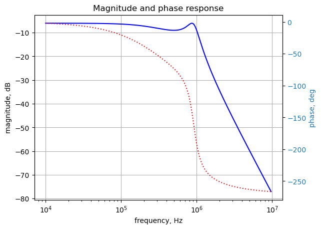

The SciPy functions square and lsim can be used to create an input squarewave and simulate the output response as shown below.

sys_tf = signal.TransferFunction(a,b)

# define the time interval and create a square wave
t = np.linspace(0, 20e-6, 1000, endpoint=False)
ref_sqr_signal = signal.square(2*np.pi*1e5*t, duty=0.5)

# call lsim to generate the response signal
ref_t_step, ref_y_step, ref_x_step = signal.lsim(sys_tf, U=ref_sqr_signal, T=t)

plt.plot(ref_t_step*1e6, ref_sqr_signal, 'r', alpha = 1.0, linewidth=1, label='$v_1(t)$')
plt.plot(ref_t_step*1e6, ref_y_step,'b', linewidth = 1.0, label='$v_2(t)$')
plt.title('Square Wave Response')
plt.ylabel('volts')
plt.xlabel('time, usec')
plt.grid()
plt.legend(loc='best')
# show plot
plt.show()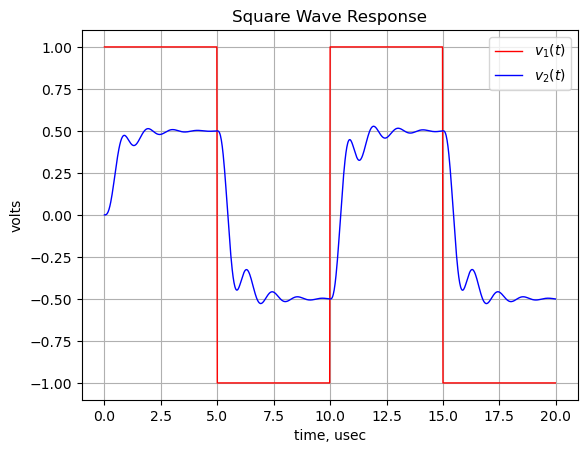

The time domain response of the filter to a square wave is early obtained and plotted. Given the filter’s design parameters, the step response shows a bit of ringing at each transition.

8.2 Circuit Example 2

Figure 8.2: Circuit schematic

The circuit in Figure 8.2 is an elliptic low pass filter with a 1 Hz cut off and 3 dB of ripple in the pass band and 40 dB of attenuation in the stop band. Three dB of ripple in the pass band was designed in so that the transient response would have some ringing. The filter design tool linked here was used to design the filter.

The netlist generated by LTSpice is pasted into the cell below and some edits were made to remove the inductor series resistance and the independent source, V1, is set to a value of one.

net_list = '''
V1 1 0 1
R1 3 1 1
R2 2 0 1
L1 3 4 0.4925
L2 5 0 0.05081
C2 4 5 0.09876
L3 4 2 0.4925
'''

Generate and display the network equations.

report, network_df, df2, A, X, Z = SymMNA.smna(net_list)

# Put matrices into SymPy 
X = Matrix(X)
Z = Matrix(Z)

NE_sym = Eq(A*X,Z)

# The symbols generated by the Python code are extracted by the SymPy function free_symbols
# and then declared as SymPy variables.
var(str(NE_sym.free_symbols).replace('{','').replace('}',''))

# built a dictionary of element values.
element_values = SymMNA.get_part_values(network_df)

# generate markdown text to display the network equations.
temp = ''
for i in range(len(X)):
    temp += '${:s}$<br>'.format(latex(Eq((A*X)[i:i+1][0],Z[i])))

Markdown(temp)

\(I_{V1} + \frac{v_{1}}{R_{1}} - \frac{v_{3}}{R_{1}} = 0\)
\(- I_{L3} + \frac{v_{2}}{R_{2}} = 0\)
\(I_{L1} - \frac{v_{1}}{R_{1}} + \frac{v_{3}}{R_{1}} = 0\)
\(C_{2} s v_{4} - C_{2} s v_{5} - I_{L1} + I_{L3} = 0\)
\(- C_{2} s v_{4} + C_{2} s v_{5} + I_{L2} = 0\)
\(v_{1} = V_{1}\)
\(- I_{L1} L_{1} s + v_{3} - v_{4} = 0\)
\(- I_{L2} L_{2} s + v_{5} = 0\)
\(- I_{L3} L_{3} s - v_{2} + v_{4} = 0\)

As shown above MNA generated many equations and these would be difficult to solve by hand.

Since the circuit is not too large, a symbolic solution can be easily obtained. The IPython magic command %%time is being used to get the length of time for the solution.

%%time
U_sym = solve(NE_sym,X)

CPU times: user 79.3 ms, sys: 0 ns, total: 79.3 ms
Wall time: 79.6 ms

Display the symbolic solution

temp = ''
for i in U_sym.keys():
    temp += '${:s} = {:s}$<br>'.format(latex(i),latex(U_sym[i]))

Markdown(temp)

\(v_{1} = V_{1}\)
\(v_{2} = \frac{C_{2} L_{2} R_{2} V_{1} s^{2} + R_{2} V_{1}}{C_{2} L_{1} L_{2} s^{3} + C_{2} L_{1} L_{3} s^{3} + C_{2} L_{1} R_{2} s^{2} + C_{2} L_{2} L_{3} s^{3} + C_{2} L_{2} R_{1} s^{2} + C_{2} L_{2} R_{2} s^{2} + C_{2} L_{3} R_{1} s^{2} + C_{2} R_{1} R_{2} s + L_{1} s + L_{3} s + R_{1} + R_{2}}\)
\(v_{3} = \frac{C_{2} L_{1} L_{2} V_{1} s^{3} + C_{2} L_{1} L_{3} V_{1} s^{3} + C_{2} L_{1} R_{2} V_{1} s^{2} + C_{2} L_{2} L_{3} V_{1} s^{3} + C_{2} L_{2} R_{2} V_{1} s^{2} + L_{1} V_{1} s + L_{3} V_{1} s + R_{2} V_{1}}{C_{2} L_{1} L_{2} s^{3} + C_{2} L_{1} L_{3} s^{3} + C_{2} L_{1} R_{2} s^{2} + C_{2} L_{2} L_{3} s^{3} + C_{2} L_{2} R_{1} s^{2} + C_{2} L_{2} R_{2} s^{2} + C_{2} L_{3} R_{1} s^{2} + C_{2} R_{1} R_{2} s + L_{1} s + L_{3} s + R_{1} + R_{2}}\)
\(v_{4} = \frac{C_{2} L_{2} L_{3} V_{1} s^{3} + C_{2} L_{2} R_{2} V_{1} s^{2} + L_{3} V_{1} s + R_{2} V_{1}}{C_{2} L_{1} L_{2} s^{3} + C_{2} L_{1} L_{3} s^{3} + C_{2} L_{1} R_{2} s^{2} + C_{2} L_{2} L_{3} s^{3} + C_{2} L_{2} R_{1} s^{2} + C_{2} L_{2} R_{2} s^{2} + C_{2} L_{3} R_{1} s^{2} + C_{2} R_{1} R_{2} s + L_{1} s + L_{3} s + R_{1} + R_{2}}\)
\(v_{5} = \frac{C_{2} L_{2} L_{3} V_{1} s^{3} + C_{2} L_{2} R_{2} V_{1} s^{2}}{C_{2} L_{1} L_{2} s^{3} + C_{2} L_{1} L_{3} s^{3} + C_{2} L_{1} R_{2} s^{2} + C_{2} L_{2} L_{3} s^{3} + C_{2} L_{2} R_{1} s^{2} + C_{2} L_{2} R_{2} s^{2} + C_{2} L_{3} R_{1} s^{2} + C_{2} R_{1} R_{2} s + L_{1} s + L_{3} s + R_{1} + R_{2}}\)
\(I_{V1} = \frac{- C_{2} L_{2} V_{1} s^{2} - C_{2} L_{3} V_{1} s^{2} - C_{2} R_{2} V_{1} s - V_{1}}{C_{2} L_{1} L_{2} s^{3} + C_{2} L_{1} L_{3} s^{3} + C_{2} L_{1} R_{2} s^{2} + C_{2} L_{2} L_{3} s^{3} + C_{2} L_{2} R_{1} s^{2} + C_{2} L_{2} R_{2} s^{2} + C_{2} L_{3} R_{1} s^{2} + C_{2} R_{1} R_{2} s + L_{1} s + L_{3} s + R_{1} + R_{2}}\)
\(I_{L1} = \frac{C_{2} L_{2} V_{1} s^{2} + C_{2} L_{3} V_{1} s^{2} + C_{2} R_{2} V_{1} s + V_{1}}{C_{2} L_{1} L_{2} s^{3} + C_{2} L_{1} L_{3} s^{3} + C_{2} L_{1} R_{2} s^{2} + C_{2} L_{2} L_{3} s^{3} + C_{2} L_{2} R_{1} s^{2} + C_{2} L_{2} R_{2} s^{2} + C_{2} L_{3} R_{1} s^{2} + C_{2} R_{1} R_{2} s + L_{1} s + L_{3} s + R_{1} + R_{2}}\)
\(I_{L2} = \frac{C_{2} L_{3} V_{1} s^{2} + C_{2} R_{2} V_{1} s}{C_{2} L_{1} L_{2} s^{3} + C_{2} L_{1} L_{3} s^{3} + C_{2} L_{1} R_{2} s^{2} + C_{2} L_{2} L_{3} s^{3} + C_{2} L_{2} R_{1} s^{2} + C_{2} L_{2} R_{2} s^{2} + C_{2} L_{3} R_{1} s^{2} + C_{2} R_{1} R_{2} s + L_{1} s + L_{3} s + R_{1} + R_{2}}\)
\(I_{L3} = \frac{C_{2} L_{2} V_{1} s^{2} + V_{1}}{C_{2} L_{1} L_{2} s^{3} + C_{2} L_{1} L_{3} s^{3} + C_{2} L_{1} R_{2} s^{2} + C_{2} L_{2} L_{3} s^{3} + C_{2} L_{2} R_{1} s^{2} + C_{2} L_{2} R_{2} s^{2} + C_{2} L_{3} R_{1} s^{2} + C_{2} R_{1} R_{2} s + L_{1} s + L_{3} s + R_{1} + R_{2}}\)

After substituting the numeric component values for the elements, a numerical solution for the note voltages can be obtained for the steady state condition.

NE = NE_sym.subs(element_values)

U = solve(NE,X)

The frequency response plot of the transfer function \(H(s)=\frac{v_2}{v_1}\) is plotted with the code below.

H = U[v2]/U[v1]

num, denom = fraction(H) #returns numerator and denominator

# convert symbolic to numpy polynomial
a = np.array(Poly(num, s).all_coeffs(), dtype=float)
b = np.array(Poly(denom, s).all_coeffs(), dtype=float)
system = (a, b)

x = np.logspace(-1, 1, 200, endpoint=False)*2*np.pi
w, mag, phase = signal.bode(system, w=x) # returns: rad/s, mag in dB, phase in deg

fig, ax1 = plt.subplots()
ax1.set_ylabel('magnitude, dB')
ax1.set_xlabel('frequency, Hz')

plt.semilogx(w/(2*np.pi), mag,'-b')    # Bode magnitude plot

ax1.tick_params(axis='y')
#ax1.set_ylim((-30,20))
plt.grid()

# instantiate a second y-axes that shares the same x-axis
ax2 = ax1.twinx()
color = 'tab:blue'

plt.semilogx(w/(2*np.pi), phase,':',color='tab:red')  # Bode phase plot

ax2.set_ylabel('phase, deg',color=color)
ax2.tick_params(axis='y', labelcolor=color)
#ax2.set_ylim((-5,25))

plt.title('Magnitude and phase response')
plt.show()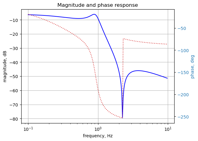

8.2.1 Transient Analysis Using Laplace Transforms

The input signal, \(V_1\), for the filter circuit can be defined by using SymPy’s Heaveside function. The signal has a positive step at t=0, followed by a return to zero amplitude at t=5.

Declare \(t\) as a SymPy symbol, which is needed for the analysis. Then use the Heaveside(t) function to construct a single rectangular pulse for \(V_1(t)\).

t = symbols('t',positive=True)  # t > 0

V1_t = 1*Heaviside(t)*(1-Heaviside(t-5))
V1_t

\(\displaystyle 1 - \theta\left(t - 5\right)\)

Use the lambdify function to convert \(V_1(t)\) to a function for plotting.

func_V1_t = lambdify(t, V1_t) 

The time domain description of the input signal is converted to the frequency domain with SymPy’s Laplace transform function.

V1_s = laplace_transform(V1_t, t, s, noconds=True)
V1_s

\(\displaystyle \frac{1}{s} - \frac{e^{- 5 s}}{s}\)

Put the component values into the network equations, set V1 equal to the Laplace of the input signal and display the equations.

element_values[V1] = V1_s
NE_trans = NE_sym.subs(element_values)

# display the equations with numeric values.
temp = ''
for i in range(shape(NE.lhs)[0]):
    temp += '${:s} = {:s}$<br>'.format(latex(NE_trans.rhs[i]),latex(NE_trans.lhs[i]))

Markdown(temp)

\(0 = I_{V1} + 1.0 v_{1} - 1.0 v_{3}\)
\(0 = - I_{L3} + 1.0 v_{2}\)
\(0 = I_{L1} - 1.0 v_{1} + 1.0 v_{3}\)
\(0 = - I_{L1} + I_{L3} + 0.09876 s v_{4} - 0.09876 s v_{5}\)
\(0 = I_{L2} - 0.09876 s v_{4} + 0.09876 s v_{5}\)
\(\frac{1}{s} - \frac{e^{- 5 s}}{s} = v_{1}\)
\(0 = - 0.4925 I_{L1} s + v_{3} - v_{4}\)
\(0 = - 0.05081 I_{L2} s + v_{5}\)
\(0 = - 0.4925 I_{L3} s - v_{2} + v_{4}\)

Notice that \(v_1=\frac{1}{s}-\frac{e^{-5s}}{s}\) in the 6th equation above.

Solve the network equations for the transient input and display the results.

%%time
U_trans = solve(NE_trans,X)

CPU times: user 2.35 s, sys: 0 ns, total: 2.35 s
Wall time: 2.35 s

temp = ''
for i in U_trans.keys():
    temp += '${:s} = {:s}$<br>'.format(latex(i),latex(U_trans[i]))

Markdown(temp)

\(v_{1} = \frac{1}{s} - \frac{e^{- 5.0 s}}{s}\)
\(v_{2} = \frac{1254498900.0 s^{2} e^{5.0 s}}{7224395229.0 s^{4} e^{5.0 s} + 26828647800.0 s^{3} e^{5.0 s} + 270940000000.0 s^{2} e^{5.0 s} + 500000000000.0 s e^{5.0 s}} - \frac{1254498900.0 s^{2}}{7224395229.0 s^{4} e^{5.0 s} + 26828647800.0 s^{3} e^{5.0 s} + 270940000000.0 s^{2} e^{5.0 s} + 500000000000.0 s e^{5.0 s}} + \frac{250000000000.0 e^{5.0 s}}{7224395229.0 s^{4} e^{5.0 s} + 26828647800.0 s^{3} e^{5.0 s} + 270940000000.0 s^{2} e^{5.0 s} + 500000000000.0 s e^{5.0 s}} - \frac{250000000000.0}{7224395229.0 s^{4} e^{5.0 s} + 26828647800.0 s^{3} e^{5.0 s} + 270940000000.0 s^{2} e^{5.0 s} + 500000000000.0 s e^{5.0 s}}\)
\(v_{3} = \frac{7224395229.0 s^{3} e^{5.0 s}}{7224395229.0 s^{4} e^{5.0 s} + 26828647800.0 s^{3} e^{5.0 s} + 270940000000.0 s^{2} e^{5.0 s} + 500000000000.0 s e^{5.0 s}} - \frac{7224395229.0 s^{3}}{7224395229.0 s^{4} e^{5.0 s} + 26828647800.0 s^{3} e^{5.0 s} + 270940000000.0 s^{2} e^{5.0 s} + 500000000000.0 s e^{5.0 s}} + \frac{13414323900.0 s^{2} e^{5.0 s}}{7224395229.0 s^{4} e^{5.0 s} + 26828647800.0 s^{3} e^{5.0 s} + 270940000000.0 s^{2} e^{5.0 s} + 500000000000.0 s e^{5.0 s}} - \frac{13414323900.0 s^{2}}{7224395229.0 s^{4} e^{5.0 s} + 26828647800.0 s^{3} e^{5.0 s} + 270940000000.0 s^{2} e^{5.0 s} + 500000000000.0 s e^{5.0 s}} + \frac{246250000000.0 s e^{5.0 s}}{7224395229.0 s^{4} e^{5.0 s} + 26828647800.0 s^{3} e^{5.0 s} + 270940000000.0 s^{2} e^{5.0 s} + 500000000000.0 s e^{5.0 s}} - \frac{246250000000.0 s}{7224395229.0 s^{4} e^{5.0 s} + 26828647800.0 s^{3} e^{5.0 s} + 270940000000.0 s^{2} e^{5.0 s} + 500000000000.0 s e^{5.0 s}} + \frac{250000000000.0 e^{5.0 s}}{7224395229.0 s^{4} e^{5.0 s} + 26828647800.0 s^{3} e^{5.0 s} + 270940000000.0 s^{2} e^{5.0 s} + 500000000000.0 s e^{5.0 s}} - \frac{250000000000.0}{7224395229.0 s^{4} e^{5.0 s} + 26828647800.0 s^{3} e^{5.0 s} + 270940000000.0 s^{2} e^{5.0 s} + 500000000000.0 s e^{5.0 s}}\)
\(v_{4} = \frac{12544989.0 s^{2} e^{5.0 s}}{146688228.0 s^{3} e^{5.0 s} + 246900000.0 s^{2} e^{5.0 s} + 5000000000.0 s e^{5.0 s}} - \frac{12544989.0 s^{2}}{146688228.0 s^{3} e^{5.0 s} + 246900000.0 s^{2} e^{5.0 s} + 5000000000.0 s e^{5.0 s}} + \frac{2500000000.0 e^{5.0 s}}{146688228.0 s^{3} e^{5.0 s} + 246900000.0 s^{2} e^{5.0 s} + 5000000000.0 s e^{5.0 s}} - \frac{2500000000.0}{146688228.0 s^{3} e^{5.0 s} + 246900000.0 s^{2} e^{5.0 s} + 5000000000.0 s e^{5.0 s}}\)
\(v_{5} = \frac{12544989.0 s e^{5.0 s}}{146688228.0 s^{2} e^{5.0 s} + 246900000.0 s e^{5.0 s} + 5000000000.0 e^{5.0 s}} - \frac{12544989.0 s}{146688228.0 s^{2} e^{5.0 s} + 246900000.0 s e^{5.0 s} + 5000000000.0 e^{5.0 s}}\)
\(I_{V1} = - \frac{13414323900.0 s^{2} e^{5.0 s}}{7224395229.0 s^{4} e^{5.0 s} + 26828647800.0 s^{3} e^{5.0 s} + 270940000000.0 s^{2} e^{5.0 s} + 500000000000.0 s e^{5.0 s}} + \frac{13414323900.0 s^{2}}{7224395229.0 s^{4} e^{5.0 s} + 26828647800.0 s^{3} e^{5.0 s} + 270940000000.0 s^{2} e^{5.0 s} + 500000000000.0 s e^{5.0 s}} - \frac{24690000000.0 s e^{5.0 s}}{7224395229.0 s^{4} e^{5.0 s} + 26828647800.0 s^{3} e^{5.0 s} + 270940000000.0 s^{2} e^{5.0 s} + 500000000000.0 s e^{5.0 s}} + \frac{24690000000.0 s}{7224395229.0 s^{4} e^{5.0 s} + 26828647800.0 s^{3} e^{5.0 s} + 270940000000.0 s^{2} e^{5.0 s} + 500000000000.0 s e^{5.0 s}} - \frac{250000000000.0 e^{5.0 s}}{7224395229.0 s^{4} e^{5.0 s} + 26828647800.0 s^{3} e^{5.0 s} + 270940000000.0 s^{2} e^{5.0 s} + 500000000000.0 s e^{5.0 s}} + \frac{250000000000.0}{7224395229.0 s^{4} e^{5.0 s} + 26828647800.0 s^{3} e^{5.0 s} + 270940000000.0 s^{2} e^{5.0 s} + 500000000000.0 s e^{5.0 s}}\)
\(I_{L1} = \frac{13414323900.0 s^{2} e^{5.0 s}}{7224395229.0 s^{4} e^{5.0 s} + 26828647800.0 s^{3} e^{5.0 s} + 270940000000.0 s^{2} e^{5.0 s} + 500000000000.0 s e^{5.0 s}} - \frac{13414323900.0 s^{2}}{7224395229.0 s^{4} e^{5.0 s} + 26828647800.0 s^{3} e^{5.0 s} + 270940000000.0 s^{2} e^{5.0 s} + 500000000000.0 s e^{5.0 s}} + \frac{24690000000.0 s e^{5.0 s}}{7224395229.0 s^{4} e^{5.0 s} + 26828647800.0 s^{3} e^{5.0 s} + 270940000000.0 s^{2} e^{5.0 s} + 500000000000.0 s e^{5.0 s}} - \frac{24690000000.0 s}{7224395229.0 s^{4} e^{5.0 s} + 26828647800.0 s^{3} e^{5.0 s} + 270940000000.0 s^{2} e^{5.0 s} + 500000000000.0 s e^{5.0 s}} + \frac{250000000000.0 e^{5.0 s}}{7224395229.0 s^{4} e^{5.0 s} + 26828647800.0 s^{3} e^{5.0 s} + 270940000000.0 s^{2} e^{5.0 s} + 500000000000.0 s e^{5.0 s}} - \frac{250000000000.0}{7224395229.0 s^{4} e^{5.0 s} + 26828647800.0 s^{3} e^{5.0 s} + 270940000000.0 s^{2} e^{5.0 s} + 500000000000.0 s e^{5.0 s}}\)
\(I_{L2} = \frac{61725000.0 e^{5.0 s}}{36672057.0 s^{2} e^{5.0 s} + 61725000.0 s e^{5.0 s} + 1250000000.0 e^{5.0 s}} - \frac{61725000.0}{36672057.0 s^{2} e^{5.0 s} + 61725000.0 s e^{5.0 s} + 1250000000.0 e^{5.0 s}}\)
\(I_{L3} = \frac{1254498900.0 s^{2} e^{5.0 s}}{7224395229.0 s^{4} e^{5.0 s} + 26828647800.0 s^{3} e^{5.0 s} + 270940000000.0 s^{2} e^{5.0 s} + 500000000000.0 s e^{5.0 s}} - \frac{1254498900.0 s^{2}}{7224395229.0 s^{4} e^{5.0 s} + 26828647800.0 s^{3} e^{5.0 s} + 270940000000.0 s^{2} e^{5.0 s} + 500000000000.0 s e^{5.0 s}} + \frac{250000000000.0 e^{5.0 s}}{7224395229.0 s^{4} e^{5.0 s} + 26828647800.0 s^{3} e^{5.0 s} + 270940000000.0 s^{2} e^{5.0 s} + 500000000000.0 s e^{5.0 s}} - \frac{250000000000.0}{7224395229.0 s^{4} e^{5.0 s} + 26828647800.0 s^{3} e^{5.0 s} + 270940000000.0 s^{2} e^{5.0 s} + 500000000000.0 s e^{5.0 s}}\)

The equations for the solution are complex and long, but are easy to obtain and display.

The voltage at node 2 is the output of the filter. The expression is simplified with the chain of operators applied to the expression: nsimplify() and simplify().

H = U_trans[v2].nsimplify().simplify()
H

\(\displaystyle \frac{100 \cdot \left(12544989 s^{2} e^{5 s} - 12544989 s^{2} + 2500000000 e^{5 s} - 2500000000\right) e^{- 5 s}}{s \left(7224395229 s^{3} + 26828647800 s^{2} + 270940000000 s + 500000000000\right)}\)

Transient analysis is somewhat more involved than the other types of circuit analysis, primarily because SymPy’s inverse Laplace transform is not very robust and can’t handle complicated expressions. The output equation needs to be simplified by writing some code to put the equation into forms that SymPy can deal with. The following procedure mostly follows what was outlined in a stackoverflow answer here.

Extract the numerator and denominator and display. All the time dealy terms are in the numerator.

n, d = fraction(H)
display('numerator', n, 'denominator', d)

'numerator'

\(\displaystyle 1254498900 s^{2} e^{5 s} - 1254498900 s^{2} + 250000000000 e^{5 s} - 250000000000\)

'denominator'

\(\displaystyle s \left(7224395229 s^{3} + 26828647800 s^{2} + 270940000000 s + 500000000000\right) e^{5 s}\)

Each of the numerator terms can be put over the common denominator.

terms = [a / d for a in n.args]
display(terms)

\(\displaystyle \left[ - \frac{250000000000 e^{- 5 s}}{s \left(7224395229 s^{3} + 26828647800 s^{2} + 270940000000 s + 500000000000\right)}, \ - \frac{1254498900 s e^{- 5 s}}{7224395229 s^{3} + 26828647800 s^{2} + 270940000000 s + 500000000000}, \ \frac{250000000000}{s \left(7224395229 s^{3} + 26828647800 s^{2} + 270940000000 s + 500000000000\right)}, \ \frac{1254498900 s}{7224395229 s^{3} + 26828647800 s^{2} + 270940000000 s + 500000000000}\right]\)

The following code processes each of the terms obtained above.

• The time delay operator \(e^{-ts}\) is removed from the expression and the value of the time delay is saved in a list.
• use the SciPy residue function to get the partial-fraction expansion residues and poles
• build the partial expansion terms and find the inverse Laplace of each one and save

time_delay = []
delay = []
N = []

for p1 in terms:
    # look for and remove the time delay
    if len(p1.find(exp)) == 1:
        delay = p1.find(exp).pop()
        time_delay.append(list(delay.atoms())[0])
        ans = p1/p1.find(exp).pop()
    else:
        ans = p1
        time_delay.append(0)

    # use the SciPy residue function to get the partial-fraction expansion residues and poles
    n, d = fraction(ans)
    cn = Poly(n, s).all_coeffs()
    cd = Poly(d, s).all_coeffs()
    r, p, k = signal.residue(cn, cd, tol=0.001, rtype='avg')
    
    # build a symbolic expression for each of the residues and find the inverse Laplace of each one and save
    z = 0
    for i in range(len(r)):
        m = (r[i]/(s-p[i])) #.nsimplify()
        z += inverse_laplace_transform(m, s, t)

    N.append(z)

The time delays associated with each term are:

time_delay

\(\displaystyle \left[ -5, \ -5, \ 0, \ 0\right]\)

The time domain version of each of the terms is displayed below.

N

\(\displaystyle \left[ 1.0 \left(\left(0.0868202525095611 - 0.00506716236561563 i\right) \sin{\left(5.77733847617481 t \right)} + \left(0.00506716236561563 + 0.0868202525095611 i\right) \cos{\left(5.77733847617481 t \right)}\right) e^{- 0.841580825422473 t} + 1.0 \left(\left(0.0868202525095611 + 0.00506716236561563 i\right) \sin{\left(5.77733847617481 t \right)} + \left(0.00506716236561563 - 0.0868202525095611 i\right) \cos{\left(5.77733847617481 t \right)}\right) e^{- 0.841580825422473 t} - 0.5 + 0.489865675268769 e^{- 2.03045685279188 t}, \ 1.0 \left(\left(-0.0139856047826648 + 0.00506716236561562 i\right) \sin{\left(5.77733847617481 t \right)} - \left(0.00506716236561562 + 0.0139856047826648 i\right) \cos{\left(5.77733847617481 t \right)}\right) e^{- 0.841580825422473 t} + 1.0 \left(- \left(0.0139856047826648 + 0.00506716236561562 i\right) \sin{\left(5.77733847617481 t \right)} + \left(-0.00506716236561562 + 0.0139856047826648 i\right) \cos{\left(5.77733847617481 t \right)}\right) e^{- 0.841580825422473 t} + 0.0101343247312312 e^{- 2.03045685279188 t}, \ 1.0 \left(\left(-0.0868202525095611 + 0.00506716236561563 i\right) \sin{\left(5.77733847617481 t \right)} - \left(0.00506716236561563 + 0.0868202525095611 i\right) \cos{\left(5.77733847617481 t \right)}\right) e^{- 0.841580825422473 t} + 1.0 \left(- \left(0.0868202525095611 + 0.00506716236561563 i\right) \sin{\left(5.77733847617481 t \right)} + \left(-0.00506716236561563 + 0.0868202525095611 i\right) \cos{\left(5.77733847617481 t \right)}\right) e^{- 0.841580825422473 t} + 0.5 - 0.489865675268769 e^{- 2.03045685279188 t}, \ 1.0 \left(\left(0.0139856047826648 - 0.00506716236561562 i\right) \sin{\left(5.77733847617481 t \right)} + \left(0.00506716236561562 + 0.0139856047826648 i\right) \cos{\left(5.77733847617481 t \right)}\right) e^{- 0.841580825422473 t} + 1.0 \left(\left(0.0139856047826648 + 0.00506716236561562 i\right) \sin{\left(5.77733847617481 t \right)} + \left(0.00506716236561562 - 0.0139856047826648 i\right) \cos{\left(5.77733847617481 t \right)}\right) e^{- 0.841580825422473 t} - 0.0101343247312312 e^{- 2.03045685279188 t}\right]\)

Each of these terms can be converted to a function using SymPy’s lambdify function.

out0 = lambdify(t, N[0])
out1 = lambdify(t, N[1])
out2 = lambdify(t, N[2])
out3 = lambdify(t, N[3])

Define the values for the x-axis of the plot and put each one into an array for plotting.

x = np.linspace(0, 10, 2000, endpoint=True)

out0a = out0(x)
out1a = out1(x)
out2a = out2(x)
out3a = out3(x)

The arrays, out2a and out3a, do not have any delay so they can be summed and used to create the final array for plotting.

out = out2a + out3a

The arrays, out0a and out1a, have a delay associated with them, so and offset in the time is included by shifting right by the correct amount.

offset = 1000
out[offset:] = out[offset:] + (out0a[0:-offset] + out1a[0:-offset])

Plot the final combined result.

plt.title('Filter output voltage vs time')

plt.plot(x, np.real(out),label='v2(t)')
plt.plot(x, np.real(func_V1_t(x)),label='V1(t)')

plt.ylabel('v(t), volts')
plt.xlabel('time, sec')

plt.legend()
plt.grid()
plt.show()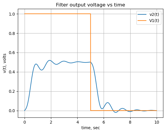

8.2.2 Transient Analysis Using SciPy

Using the expression for the steady state solution obtained above, we can use SciPy to plot the transient response to a square wave.

H = U[v2]/U[v1]

num, denom = fraction(H) #returns numerator and denominator

# convert symbolic to numpy polynomial
a = np.array(Poly(num, s).all_coeffs(), dtype=float)
b = np.array(Poly(denom, s).all_coeffs(), dtype=float)
system = (a, b)

sys_tf = signal.TransferFunction(a,b)

# define the time interval and create a square wave
t = np.linspace(0, 10, 1000, endpoint=False)
ref_sqr_signal = signal.square(2*np.pi*1e-1*t, duty=0.5)

# call lsim to generate the response signal
ref_t_step, ref_y_step, ref_x_step = signal.lsim(sys_tf, U=ref_sqr_signal, T=t)

plt.plot(ref_t_step, ref_sqr_signal, 'r', alpha = 1.0, linewidth=1, label='$v_1(t)$')
plt.plot(ref_t_step, ref_y_step,'b', linewidth = 1.0, label='$v_2(t)$')
plt.title('Square Wave Response')
plt.ylabel('volts')
plt.xlabel('time, sec')
plt.grid()
plt.legend(loc='best')
# show plot
plt.show()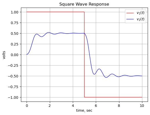

8.3 Summary

This chapter provided an overview of Transient Analysis in electrical circuits using Python-based symbolic and numerical tools. It contrasts steady-state behavior with the transient interval governed by energy-storage elements (inductors and capacitors).

The transient response as seen with a square wave input was explored. In circuit example 2, the inverse Laplace transform of complicated expressions requires that they be reduced to a set of simple terms by partial fraction expansion.

8.3.1 Key Takeaways

• Laplace Transform: Used to convert differential equations into algebraic ones, represented as for a unit step in the frequency domain.
• Step Response: A critical performance benchmark used to measure rise time, overshoot, and settling time.
• Computational Efficiency: While manual MNA is labor-intensive, Python libraries like SymMNA and SymPy can solve complex symbolic matrices in milliseconds.
• Inverse Laplace Challenges: For higher-order systems (like the Elliptic filter), manual decomposition into partial fractions or numerical methods (SciPy.signal.lsim) is often more robust than a direct symbolic Inverse Laplace approach.
• Predictive Power: The Step Response is the “DNA” of the circuit; knowing it allows engineers to predict how the system will react to any complex input signal. In engineering and control theory, the “Step Response” is often considered one of the most informative test you can perform on a system.

Marki Microwave. 2025. “LC Filter Design Tool.” Marki Microwave. 2025. https://markimicrowave.com/technical-resources/tools/lc-filter-design-tool/.