2 Basic Concepts

This chapter will cover some fundamental concepts and definitions related to electric circuit analysis are presented.

Electric circuit analysis relies on fundamental concepts starting with Ideal Components, which are theoretical models (like a perfect resistor or capacitor) that simplify analysis by ignoring real-world imperfections. These components are connected to form a circuit, which is represented visually by a Schematic and algebraically by a Netlist. The foundational physical quantities are Electric Charge (measured in Coulombs, C), whose movement constitutes Current (Amperes, A), and Voltage (Volts, V), which represents the energy per unit charge available to move current. The core relationship between these quantities in a resistive element is defined by Ohm’s Law (\(V = IR\)). Elements are classified as Passive (resistors, capacitors, inductors) if they only consume or store energy, or Active (sources, transistors) if they generate or control energy. Finally, Energy Storage Elements. the capacitor and inductor, introduce dynamic behavior, as they store energy in electric and magnetic fields, respectively, leading to time-varying currents and voltages.

2.1 What is an Electric Circuit?

An electric circuit is a complete, closed-loop path through which electric current (a flow of electric charge) can continuously travel.

A simple circuit usually contain three fundamental parts: a power source (like a battery) to provide the energy and voltage difference needed to push the current, conductors (like wires) to carry the current, and a load (like a light bulb or motor) that uses the electrical energy and converts it into another form, such as light or motion. For the circuit to be functional, this path must remain unbroken, also known as a closed circuit; any break, like an open switch, creates an open circuit and stops the flow of current.

Electromotive Force (EMF), symbolized as \(E\) and measured in volts \(V\), is the total electrical energy provided by a source, such as a battery, generator, or solar cell, per unit of electric charge to drive current through a circuit. Although it contains the word “force”, EMF is technically a measure of energy conversion.

The source converts non-electrical energy (like chemical or mechanical) into electrical energy, thereby creating the potential difference necessary to push charge carriers around the loop. In an ideal source with no internal resistance, the EMF is equal to the terminal voltage, but in real devices, the actual voltage delivered to the external circuit is slightly less than the EMF due to the internal resistance of the source.

In electromagnetism and electronics, electromotive force is an energy transfer to an electric circuit per unit of electric charge, measured in volts.

Devices called electrical transducers provide an emf by converting other forms of energy into electrical energy. Other types of electrical equipment also produce an emf, such as batteries, which convert chemical energy, and generators, which convert mechanical energy. This energy conversion is achieved by physical forces applying physical work on electric charges.

However, electromotive force itself is not a physical force, and ISO/IEC standards have deprecated the term in favor of source voltage or source tension instead.

2.2 Electric Charge and Current

The differences between electric charge, electrical current (conventional current), and electron flow are a source of confusion for many beginners in electronics.

Here is a breakdown of the three concepts and their relationships:

1. Electric Charge (\(Q\))

Electric charge is the most fundamental concept, a physical property of matter that causes it to experience a force when placed in an electromagnetic field.
What it is: The property of subatomic particles—specifically, the protons (positive charge) and electrons (negative charge) that allows them to interact electrically.
Unit: The Coulomb. The charge on a single electron is \(1.602 \times 10^{-19} \text{ C}\).
Relationship to the others: Charge is the thing that moves to create a current. Both conventional current and electron flow describe the movement of this charge.

2. Electrical Current (Conventional Current)

Electrical current (or Conventional Current) is the standard definition used in almost all circuit analysis and engineering.
What it is: The rate of flow of electric charge through a conductor. \(I = \frac{\Delta Q}{\Delta t}\)
Unit: The Ampere, which is equivalent to one Coulomb per second.
Direction: Positive to Negative (from the positive terminal of a battery to the negative terminal).
Basis: This direction is a historical convention established by Benjamin Franklin before the discovery of the electron. He incorrectly assumed that electricity flowed from positive to negative.
Use in Circuits: This convention is almost universally used in circuit diagrams, textbooks, and Kirchhoff’s Laws, because it’s consistent whether the moving charge is positive (like ions in an electrolyte) or negative (like electrons in a wire).

3. Electron Flow

Electron flow describes the actual physical movement of the primary charge carriers in metallic conductors (like copper wire).
What it is: The physical movement of negatively charged electrons through a circuit.
Direction: Negative to Positive (from the negative terminal of a battery to the positive terminal).
Basis: This direction is based on the physical reality that electrons are the mobile charge carriers in most metal conductors, and they are repelled by the negative terminal and attracted to the positive terminal.
Use in Circuits: This model is typically used when studying the internal physics of materials, such as semiconductors, where understanding the movement of both electrons and ‘holes’ (the absence of an electron, treated as a positive charge) is crucial.

The fundamental difference lies in the direction of flow.

Feature	Electric Charge (\(Q\))	Electrical Current (Conventional Current) (\(I\))	Electron Flow
Concept	Fundamental property of matter (the stuff that moves).	Rate of charge flow (the measurement of movement).	Actual movement of charge carriers in most metal wires (the reality of movement).
Direction	N/A (Property)	Positive to Negative	Negative to Positive
Basis	Physical property of particles (protons/electrons).	Historical convention.	Physical reality of electron movement.
Primary Use	Calculating total charge (Coulombs).	Circuit analysis, schematics, engineering.	Semiconductor physics, some technician training.

In summary, Charge is the entity, Conventional Current is the agreed-upon direction used for mathematics and design (positive to negative), and Electron Flow is the true physical direction of electrons in a wire (negative to positive). Both current models lead to the same functional results in circuit calculations.

2.3 Voltage, Energy and Power

Voltage, also known as (electrical) potential difference is the difference in electric potential between two points. In the context of circuit analysis, the fundamental quantities are current, voltage and resistance.

Quantity	Unit (SI)	Symbol	Defines/Measures
Electric Current	Ampere	A (or \(I\))	The rate of flow of electric charge.
Electric Potential Difference (Voltage)	Volt	V (or \(E\) or \(U\))	The electrical “pressure” that drives the current.
Electrical Resistance	Ohm	\(\Omega\) (Omega)	The opposition a material offers to the flow of electric current.

These three units are intrinsically linked by Ohm’s Law: \(V = I \times R\).

Beyond the core three, several other quantities are crucial in circuit analysis:

Quantity	Unit (SI)	Symbol	Relationship/Formula	Measures
Electric Power	Watt	W	\(P = V \times I\)	The rate at which electrical energy is transferred or converted.
Capacitance	Farad	F	\(C = Q / V\)	A component’s ability to store an electric charge.
Inductance	Henry	H	\(V = L \frac{di}{dt}\)	A conductor’s ability to oppose a change in current.
Frequency	Hertz	Hz	\(Hz = s^{-1}\)	The number of cycles (e.g., of an AC waveform) per second.
Electrical Energy	Joule (or kWH for practical use)	J (or kWh)	\(E = P \times t\)	The work done by electrical forces.

These three concepts - Voltage, Energy, and Power - are fundamental to understanding how electricity works and are closely related. Think of electricity in terms of a water analogy to help clarify their roles:

Voltage is the electric pressure or “push” that causes electric charge (current) to flow. It is the measure of potential energy per unit charge between two points in a circuit.

Definition: The work or energy required to move a unit of electric charge from one point to another.
Symbol: \(V\)
Unit: Volt (\(\text{V}\))
\(1 \text{ Volt} = 1 \text{ Joule per Coulomb}\) (\(1 \text{ V} = 1 \text{ J/C}\))
Water Analogy: The height or pressure of the water in a tank. The higher the tank, the more pressure there is to push the water out.

Energy is the total capacity to do work. In an electrical circuit, it’s the total work done by the movement of charge.

Definition: The total amount of electrical work performed or stored. It does not have a time component.
Symbol: \(E\) or \(W\) (for Work)
Unit: Joule (\(\text{J}\)) or kilowatt-hour (\(\text{kWh}\)) for utility billing.
Water Analogy: The total volume of water in the tank. This is the total potential to do work (like filling buckets).

Key Relationship: Electrical energy (\(E\)) is simply Power (\(P\)) multiplied by the time (\(t\)) over which the power is consumed: \[E = P \times t\]

Power is the rate at which electrical energy is transferred or consumed. It tells you how quickly the work is being done.

Definition: The rate at which energy is transferred or transformed. It is energy per unit of time.
Symbol: \(P\)
Unit: Watt (\(\text{W}\))
- \(1 \text{ Watt} = 1 \text{ Joule per Second}\) (\(1 \text{ W} = 1 \text{ J/s}\))
Water Analogy: The flow rate of the water coming out of the hose (e.g., gallons per second).

Key Relationship: Electrical power is the product of Voltage (\(V\)) and Current (\(I\)): \[P = V \times I\] Power is high if you have a high voltage and a large current, or a very high voltage and a small current (as long as their product is large).

Summary of Differences

The table below summarizes the key distinctions between these three concepts:

Concept	What It Is	How It’s Measured	Relationship to Time
Voltage (\(V\))	Electric “pressure” or potential to move charge.	Volts (\(\text{V}\))	Independent of time.
Energy (\(E\))	Total work done or available to be done.	Joules (\(\text{J}\)) or \(\text{kWh}\)	Depends on the duration of time.
Power (\(P\))	Rate of energy transfer (how fast work is done).	Watts (\(\text{W}\))	Depends on instantaneous rate of change (energy per second).

2.4 Ideal Components

Ideal components are theoretical abstractions used in circuit analysis that represent perfect behavior without the imperfections of real-world components.

Component	Ideal Property	Real-World Imperfection
Resistor	Constant resistance, no inductance or capacitance.	Resistance changes with temperature.
Capacitor	Stores charge with no resistance or leakage current.	Has a small equivalent series resistance (ESR).
Inductor	Stores energy in a magnetic field with no resistance.	Has a small internal winding resistance.
Voltage Source	Provides a constant voltage regardless of the current drawn.	Has internal resistance, causing voltage to drop under load.

Ideal components are used primarily for simplification and education. By assuming perfect behavior, engineers can derive simpler mathematical models and establish foundational laws (like Ohm’s Law) that clearly illustrate the circuit’s core principles. This makes initial analysis and hand calculations much easier, providing a strong starting point before factoring in non-ideal effects for a more precise real-world design.

2.5 Schematics and Netlists

A schematic is the graphical blueprint of an electronic circuit. It uses standardized symbols for components (resistors, batteries, etc.) and lines to visually represent the electrical connections, or nets, between them. The schematic captures the logical and functional connectivity of the circuit, illustrating how signals flow and components interact, but it does not represent the physical layout or size of the components.

In this book the Schematics and netlists were drawn and generated with LTSpice. In almost all cases, the nodes have been manually labeled using “Net Name” symbol. The netlist captures the fundamental connectivity - the “what connects to what” - without worrying about the physical location or visual aesthetics (which are handled by the layout and schematic tools, respectively).

A netlist is a text-based data structure generated from the schematic. Instead of a drawing, it is a sequential listing that describes all the component connections in a structured format. It lists the components, their unique identifiers (reference designators), their pins and which specific nets they are connected to.

In simple terms, it’s a list of all the electronic components (resistors, capacitors, voltage source etc.) in a circuit and a list of the nodes connected to their terminals. Each line of a netlist typically provides three pieces of information:

Components (Instances): A list of every part used in the circuit, usually by its reference designator (e.g., \(R_1\), \(C_3\), \(L_5\)).
Terminals: The specific connection points on each component (e.g., pin 1 and pin 2 of \(R_5\)).
Component Value: The value of the component (e.g., \(5k\)).

For example, the netlist for Figure 2.1 (exported from LTSpice) looks like this:

* \Fig_9-16.asc
V1 1 0 1 AC 1
R1 1 2 3.349k
C1 2 0 27.24p
C2 2 3 0.9085p
C3 3 0 26.77p
C4 3 4 0.4578p
C5 4 0 27.1p
C6 4 5 0.5742p
R2 5 0 10.317k
L1 2 0 1µ
L2 3 0 1µ
L3 4 0 1µ
L4 5 0 1µ
C7 5 0 27.57p
.ac lin 200 27e6 33e6
.backanno
.end

The netlist above was generated from the schematic shown in the figure below.

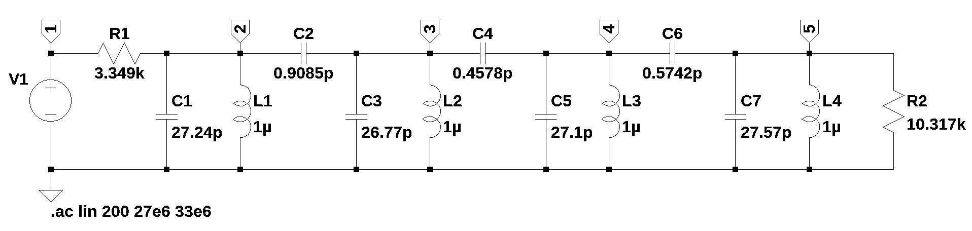
This circuit comes from Zverev (1967), Figure 9.16, which is the lumped element representation of a helical filter which has a Center frequency of 30 MHz and a - 3dB band width of approx 1MHz.

Table 2.1 shows each line of the netlist along with an explanantion. A SPICE netlist, often called a SPICE deck, is a plain-text file that describes an electronic circuit’s topology, component values, and simulation instructions for processing by a SPICE-based simulator. The “deck” terminology is a legacy of the era when circuit descriptions were fed into mainframe computers using physical punched cards. Every netlist must follow a specific structural order: the first line is the title and is ignored by SPICE, since the first character on the line is “*“, which makes the line a comment line. The last line is the .end directive. Between these, the file contains”instance lines” for components (like resistors and transistors), “dot commands” for simulation control (like .tran or .ac).

Each line as the format:

Aname node1 node 2 <node3 … > <value1 … >

The format of a standard device line is highly structured and typically follows this sequence:

Reference Designator: The first character of the line identifies the component type (e.g., R for resistor and C for capacitor).
Nodes: The next set of alphanumeric strings defines the “nets” or connection points. For example, a resistor line lists two nodes, while an Op Amp has three. Node 0 is strictly reserved for the global ground.
Value: For passive components, this is the numerical value which can have a scale factor. The Python MNA code requires numerical values without the scale factor.
Optional Parameters: Additional characteristics like temperature coefficients or initial conditions can be appended to the end of the line.

Table 2.1: LTSpice netlist

line #	LTSpice netlist lines	Explanation	Edited netlist
1	*\Fig_9-16.asc	Title of the netlist, file name
2	V1 1 0 1 AC 1	Voltage source, 1 volt DC and 1 volt AC	V1 1 0 1
3	R1 1 2 3.349k	Resistor between nodes 1 &2 of value 349k	R1 1 2 3.349e3
4	C1 2 0 27.24p	Capacitor between nodes 2 & ground of value 27.24pF	C1 2 0 27.24e-12
5	C2 2 3 0.9085p	Capacitor between nodes 2 & 3 of value 0.9085pF	C2 2 3 0.9085e-12
6	C3 3 0 26.77p	Capacitor between nodes 3 & ground of value 26.77pF	C3 3 0 26.77e-12
7	C4 3 4 0.4578p	Capacitor between nodes 3 & 4 of value 0.4578pF	C4 3 4 0.4578e-12
8	C5 4 0 27.1p	Capacitor between nodes 4 & ground of value 27.1pF	C5 4 0 27.1e-12
9	C6 4 5 0.5742p	Capacitor between nodes 4 & 5 of value 0.5742pF	C6 4 5 0.5742e-12
10	R2 5 0 10.317k	Resistor between nodes 1 &2 of value 10.317k	R2 5 0 10.317e3
11	L1 2 0 1µ	Inductor between nodes 2 and ground of value 1uH	L1 2 0 1e-6
12	L2 3 0 1µ	Inductor between nodes 3 and ground of value 1uH	L2 3 0 1e-6
13	L3 4 0 1µ	Inductor between nodes 4 and ground of value 1uH	L3 4 0 1e-6
14	L4 5 0 1µ	Inductor between nodes 5 and ground of value 1uH	L4 5 0 1e-6
15	C7 5 0 27.57p	capacitor between nodes 5 & ground of value 27.57pF	C7 5 0 27.57e-12
16	.ac lin 200 27e6 33e6	SPICE directive use to set up AC analysis
17	.backanno	SPICE directive to view a graph of the current flowing into that pin
18	.end	SPICE directive used to mark the end of the file

The netlist generated by LTSpice usually needs a bit of editing to replace the scale factors (e.g. \(\mu, k, p \text{ etc.}\)) with the numerical values as shown in the last column of Table 2.1 and shown below. Only the component lines are used by the Python MNA code.

V1 1 0 1
R1 1 2 3.349e3
C1 2 0 27.24e-12
C2 2 3 0.9085e-12
C3 3 0 26.77e-12
C4 3 4 0.4578e-12
C5 4 0 27.1e-12
C6 4 5 0.5742e-12
R2 5 0 10.317e3
L1 2 0 1e-6
L2 3 0 1e-6
L3 4 0 1e-6
L4 5 0 1e-6
C7 5 0 27.57e-12

2.6 Conventions

The following conventions are used in this book. Expressions generated by SymPy that have imaginary quantities will use \(i\) for the imaginary number. Typically, electrical engineers will use \(j\) for the imaginary number since \(i\) is the variable used for electrical current. Depending on who generates the equation, either \(i\) or \(j\) might be used and the reader should short these out based on context. Usually, the variables used for current have a number, e.g. \(i_1\) or \(i_2\) and a lone \(i\) would be the imaginary number.

The Laplace variable, \(s=j\omega\), and the one letter abbreviation for seconds, \(s\) use the same letter. It should be clear from the context whether “s” is being used for time or radian frequency.

The conventions used in this book are designed to ensure clarity and consistency in presenting circuit analysis concepts and their implementation in Python. The book adopts standard electrical engineering practices, such as representing voltages using the symbol \(V \text{ or } v\) and currents using \(I \text{ or } i\).

The sign convention for current - where current flows into the positive terminal of a passive element (like a resistor) - is a critical convention for ensuring the correct formulation of Kirchhoff’s Laws.

When translating circuits into netlists, the variables used in the symbolic and numerical calculations (like \(R_1\), \(C_2\), \(V_{source}\)) directly map to the component reference designators shown in the circuit schematics.

I’ve tried to be consistent with the use of variable names throughout the JupyterLab notebooks. Resistors, capacitors and inductors use R, L and C as reference designators. The names chosen for the other variables are listed in Table G.2

2.7 Circuit Laws

Move text from resistive circuits and RLC circuits here.

Ohm’s Law: This law states that the current flowing through a resistor is directly proportional to the voltage across it and inversely proportional to its resistance. The mathematical representation is: \(V = IR\), where:
- \(V\) is the voltage (potential difference) measured across the resistor (in Volts).
- \(I\) is the current flowing through the resistor (in Amperes).
\(R\) is the resistance of the element (in Ohms, \(\Omega\)).

Kirchhoff’s circuit laws are two equalities that deal with the current and potential difference (commonly known as voltage) in the lumped element model of electrical circuits. They were first described in 1845 by German physicist Gustav Kirchhoff.[1] This generalized the work of Georg Ohm and preceded the work of James Clerk Maxwell. Widely used in electrical engineering, they are also called Kirchhoff’s rules or simply Kirchhoff’s laws. These laws can be applied in time and frequency domains and form the basis for network analysis.

Both of Kirchhoff’s laws can be understood as corollaries of Maxwell’s equations in the low-frequency limit. They are accurate for DC circuits, and for AC circuits at frequencies where the wavelengths of electromagnetic radiation are very large compared to the circuits.

Kirchhoff’s Laws: These laws provide a framework for analyzing more complex circuits:
- Kirchhoff’s Current Law (KCL): The total current entering a junction (or node) must equal the total current leaving that junction. This is a statement of the conservation of charge.
Kirchhoff’s Voltage Law (KVL): The sum of all the voltage drops around any closed loop in a circuit must equal zero. This reflects the conservation of energy.

The analysis of electric circuits relies on fundamental laws that govern the behavior of voltage and current. The most basic is Ohm’s Law, which establishes the relationship between voltage (\(V\)), current (\(I\)), and resistance (\(R\)), stating that the voltage across a conductor is directly proportional to the current flowing through it, often expressed as \(V = IR\).

For more complex circuits, Kirchhoff’s Laws are essential: Kirchhoff’s Current Law (KCL), based on the conservation of electric charge, dictates that the sum of currents entering any junction (node) must equal the sum of currents leaving that junction (\(\sum I_{in} = \sum I_{out}\)).

Similarly, Kirchhoff’s Voltage Law (KVL), based on the conservation of energy, states that the algebraic sum of all potential differences (voltages) around any closed path (loop) in a circuit must be zero (\(\sum V = 0\)).

Together, these laws provide the necessary framework for calculating and predicting the electrical quantities in any circuit configuration.

2.8 Node and Loop Analysis

Node and Loop Analysis are two fundamental techniques used in electrical circuit analysis to determine unknown voltages and currents. Node Analysis (also known as the Nodal Voltage Method) applies Kirchhoff’s Current Law (KCL) - the algebraic sum of currents entering a node is zero - to all nodes in a circuit, except the reference node (ground). The unknowns in this method are the node voltages, which are solved by setting up a system of linear equations based on KCL.

In contrast, Loop Analysis (or the Mesh Current Method) uses Kirchhoff’s Voltage Law (KVL) - the algebraic sum of voltages around any closed loop (mesh) is zero - to find unknown mesh currents. A system of linear equations is established by applying KVL around each independent loop in the circuit.

Choosing between the two often depends on the circuit’s structure: Node Analysis is generally easier when the number of essential nodes is less than the number of independent loops, and vice versa.

2.9 Modified Nodal Analysis

Modified Nodal Analysis (MNA) is an advanced circuit analysis technique used primarily in computer-aided design (CAD) tools like SPICE to overcome the limitations of standard Nodal Analysis. While standard nodal analysis only solves for node voltages by applying Kirchhoff’s Current Law (KCL), it struggles with components where the current isn’t easily expressed as a function of node voltages, notably ideal voltage sources and inductors. MNA addresses this by including the unknown branch currents through these specific components as additional variables in the system of equations. This results in a larger but more comprehensive matrix equation, combining KCL equations for the circuit nodes with the constitutive relations (e.g., \(V = E\) for a voltage source) for the added current variables. This systematic approach allows for the efficient formulation and solution of linear and nonlinear circuit equations, making it essential for robust circuit simulation.

2.10 Laplace Transformed Circuit Elements

Laplace transformed circuit elements are a powerful method used in electrical engineering to analyze complex linear circuits, especially those with energy storage elements (inductors and capacitors) and time-varying inputs. This method converts the circuit from the time domain (\(t\)) into the s-domain (a complex frequency domain) using the Laplace transform.

Pierre-Simon, Marquis de Laplace (1749 - 1827), was an immensely influential French polymath, often referred to as the “French Newton” for his foundational work in celestial mechanics, which mathematically demonstrated the long-term stability of the solar system based on Newtonian gravity. His wide-ranging contributions also revolutionized probability theory and mathematical physics.

Among his many mathematical tools, the Laplace transform is an integral transform that converts a function of a real variable (like time, \(t\)) into a function of a complex variable (often \(s\), in the frequency domain). This transformation converts linear differential equations into simpler algebraic equations, which are much easier to solve, making the Laplace transform a crucial technique in physics and engineering, particularly for analyzing linear time-invariant systems like electrical circuits and control systems.

The key benefit is that it transforms the calculus-based equations (differential and integral equations) that describe circuit behavior into simple algebraic equations, which are much easier to solve.

The Laplace transform is a mathematical operation defined by an integral that takes a time-domain function \(f(t)\) to an s-domain function \(F(s)\): \[\mathcal{L}\{f(t)\} = F(s)\]

From Differential Equations to Algebraic Equations

In the time domain, circuits with L’s and C’s are described by differential equations. For instance, the voltage across an inductor is \(v_L(t) = L \frac{di_L(t)}{dt}\).
When transformed to the s-domain, differentiation becomes simple multiplication by \(s\), and integration becomes division by \(s\). This makes standard circuit analysis techniques (like nodal or mesh analysis) applicable using only algebra.

Element Models in the s-Domain

The time-domain components are replaced by their \(s\)-domain equivalents, including their initial conditions (like initial current \(i_L(0)\) or initial voltage \(v_C(0)\)).

Time-Domain Element	V-I Relationship	s-Domain Impedance (\(Z(s)\))
Resistor (R)	\(v_R(t) = R i_R(t)\)	\(Z_R(s) = R\)
Inductor (L)	\(v_L(t) = L \frac{di_L(t)}{dt}\)	\(Z_L(s) = sL\)
Capacitor (C)	\(i_C(t) = C \frac{dv_C(t)}{dt}\)	\(Z_C(s) = \frac{1}{sC}\)

In the s-domain, the Inductor and Capacitor are modeled as complex impedances dependent on the complex frequency \(s\).

Applications of s-Domain Models

Using the Laplace transform provides several powerful analytical tools:

Transient Response: It easily solves for the circuit’s complete response—both the transient (short-term switching behavior) and steady-state (long-term) response, especially for non-sinusoidal inputs like step or impulse functions.
Transfer Function: The ratio of the output voltage/current transform to the input voltage/current transform gives the circuit’s Transfer Function, \(H(s)\). \[H(s) = \frac{\text{Output}(s)}{\text{Input}(s)}\] This single function contains all the information needed to analyze the system’s stability, frequency response, and transient behavior (via its poles and zeros).
Initial Conditions: The transformation naturally incorporates the circuit’s initial energy storage (non-zero initial currents or voltages) as independent voltage or current sources in the s-domain equivalent circuit.

The resulting solution \(V(s)\) or \(I(s)\) is then converted back to the time domain \(v(t)\) or \(i(t)\) using the inverse Laplace transform.

2.11 Python and JupyterLab

Python and JupyterLab are two fundamental tools in modern data science and software development workflows. Python is a highly versatile, high-level, interpreted programming language known for its readability and extensive ecosystem of libraries (like NumPy, Pandas, and Matplotlib). It serves as the primary language for writing code, performing analysis and building applications.

JupyterLab, on the other hand, is a web-based interactive development environment (IDE) that provides a flexible interface for working with Jupyter Notebooks, code and data. It allows users to combine live Python code, narrative text (Markdown), equations (LaTeX), and visualizations into a single, shareable document, making it an ideal environment for exploratory data analysis, data cleaning, statistical modeling, and documentation. Together, Python’s power and JupyterLab’s interactive capabilities create a seamless and productive platform for computational tasks.

SymPy is an open-source Python library dedicated to symbolic mathematics, aiming to become a full-featured computer algebra system (CAS) while maintaining a simple, extensible code base. Unlike standard numerical libraries like NumPy, which calculate approximate decimal values, SymPy performs computations on mathematical objects exactly. It provides a wide range of capabilities, including polynomial simplification, calculus (limits, derivatives, and integrals), linear algebra, and solving differential equations, all within a native Python environment.

NumPy, short for Numerical Python, is the fundamental library for scientific computing in Python. It provides a high-performance multidimensional array object and a comprehensive collection of functions for performing fast operations on these arrays, including mathematical, logical, shape manipulation, sorting, and linear algebra.

SciPy is an open-source Python library used primarily for scientific and technical computing, building directly upon the foundational array structures of NumPy. It provides a massive collection of high-level functions and mathematical algorithms designed to handle complex tasks like numerical integration, linear algebra, optimization, signal processing, and statistics. Because it is highly optimized and written in low-level languages like C and Fortran, SciPy allows researchers and engineers to perform heavy-duty computations with the ease of Python’s syntax while maintaining near-native execution speeds. It is a core component of the “scientific Python stack,” serving as the bridge between basic data manipulation and advanced domain-specific analysis.